Tutorials for k-means clustering inference
Tutorials.RmdIn this tutorial, we demonstrate basic use of the CADET
package for testing for a difference in feature means between clusters
obtained via k-means clustering.
First we load relevant packages:
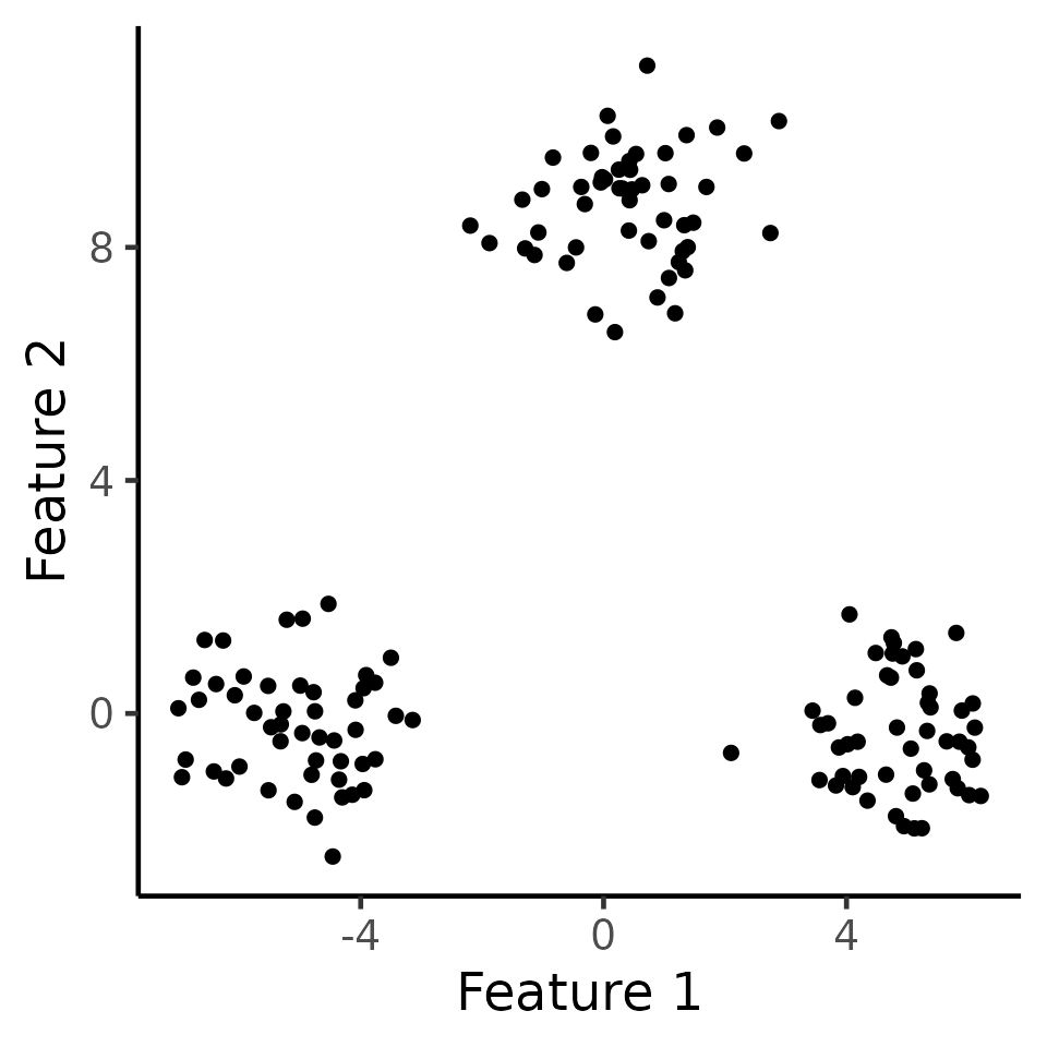
We first generate data according to \(\mathbf{X} \sim MN_{n\times q}(\boldsymbol{\mu}, \textbf{I}_n, \sigma^2 \textbf{I}_q)\) with \(n=150,q=2,\sigma=1,\) and \[\begin{align} \label{eq:power_model} \boldsymbol{\mu}_1 =\ldots = \boldsymbol{\mu}_{50} = \begin{bmatrix} -\delta/2 \\ 0_{q-1} \end{bmatrix}, \; {\boldsymbol\mu}_{51}=\ldots = \boldsymbol{\mu}_{100} = \begin{bmatrix} 0_{q-1} \\ \sqrt{3}\delta/2 \end{bmatrix} ,\; \boldsymbol{\mu}_{101}=\ldots = \boldsymbol{\mu}_{150} = \begin{bmatrix} \delta/2 \\ 0_{q-1} \end{bmatrix}. \end{align}\] Here, we can think of \(C_1 = \{1,\ldots,50\},C_2 = \{51,\ldots,100\},C_3 = \{101,\ldots,150\}\) as the “true clusters”. In the figure below, we display one such simulation \(\mathbf{x}\in\mathbb{R}^{100\times 2}\) with \(\delta=10\).
set.seed(2022)
n <- 150
true_clusters <- c(rep(1, 50), rep(2, 50), rep(3, 50))
delta <- 10
q <- 2
mu <- rbind(c(delta / 2, rep(0, q - 1)), c(rep(0, q - 1), sqrt(3) * delta / 2), c(-delta / 2, rep(0, q - 1)))
sig <- 1
X <- matrix(rnorm(n * q, sd = sig), n, q) + mu[true_clusters, ]

ggplot(data.frame(X), aes(x = X1, y = X2)) +
  geom_point(cex = 2) +
  xlab("Feature 1") +
  ylab("Feature 2") +
  theme_classic(base_size = 18) +
  theme(legend.position = "none") +
  scale_colour_manual(values = c("dodgerblue3", "rosybrown", "orange")) +
  theme(
    legend.title = element_blank(),
    plot.title = element_text(hjust = 0.5)
  )
k-means clustering (K=3)
In the code below, we call the kmeans_estimation
function to estimate clusters using Lloyd’s algorithm with \(K=3\). In the figure below, observations
are colored by the clusters obtained via \(k\)-means clustering with \(K=3\). In this case, \(k\)-means recovers the true clusters
perfectly.
k <- 3
estimated_clusters <- kmeans_estimation(X, k, iter.max = 20, seed = 2021)$final_cluster
table(true_clusters, estimated_clusters)
#>              estimated_clusters
#> true_clusters  1  2  3
#>             1  0 50  0
#>             2  0  0 50
#>             3 50  0  0
ggplot(data.frame(X), aes(x = X1, y = X2, col = as.factor(estimated_clusters))) +
  geom_point(cex = 2) +
  xlab("Feature 1") +
  ylab("Feature 2") +
  theme_classic(base_size = 18) +
  theme(legend.position = "none") +
  scale_colour_manual(values = c("dodgerblue3", "rosybrown", "orange")) +
  theme(
    legend.title = element_blank(),
    plot.title = element_text(hjust = 0.5)
  )
The kmeans_estimation function implements the Lloyd’s
algorithm for k-means clustering and stores all the intermediate
clustering assignments. The estimated clusters via
kmeans_estimation, as well as their orders, agree
with the those returned by the kmeans function in base
R when specifying algorithm = "Lloyd".
N.B.: the kmeans function in base R is
implemented in Fortran and C, while our implementation is entirely in
R. As a result, these two functions might disagree on few
corner cases.
Inference for a single feature mean after k-means clustering
In this section, we demonstrate how to use our software to obtain
\(p\)-values for testing for a
difference in the means of a single feature between a pair of clusters
identified via \(k\)-means clustering.
As an example, consider testing for a difference in the first feature (x
axis) between the orange cluster (labeled as 2 in
estimated_clusters) and the pink cluster (labeled as 3 in
estimated_clusters).
The code below demonstrates how to use the function
kmeans_inference_1f, which performs inference on the
specified two estimated clusters. After obtaining the inferential
result, we call the summary method to get a summary of the results, in
the form of a data frame.
cluster_1 <- 2
cluster_2 <- 3
cl_inference_demo <- kmeans_inference_1f(X,
  k = 3, cluster_1, cluster_2,
  feat = 1, iso = TRUE,
  sig = sig,
  covMat = NULL, seed = 2021,
  iter.max = 30
)
summary(cl_inference_demo)
#>   cluster_1 cluster_2 test_stat  p_selective       p_naive
#> 1         2         3  4.464756 8.514513e-29 2.171388e-110
In the summary, we have the empirical difference in means of the
second feature between the two clusters, i.e.,\(\sum_{i\in \hat{G}}\mathbf{x}_{i,2}/|\hat{{G}}| -
\sum_{i\in \hat{G}'}\mathbf{x}_{i,2}/|\hat{G}'|\)
(test_stats), the naive p-value based on a z-test
(p_naive), and the selective \(p\)-value (p_selective). In
this case, the test based on \(p_{\text{selective}}\) can reject this null
hypothesis that the blue and pink clusters have the same mean in the
first feature (\(p_{2,\text{selective}}<0.001\)).
Inference for k-means clustering when the null hypothesis holds
In this section, we demonstrate that our proposed \(p\)-value yields reasonable results when the null hypothesis does hold. Consider the same data as before, and we apply \(k\)-means clustering with \(K=4\) to obtain four estimated clusters.
k_new <- 4
new_estimated_clusters <- kmeans_estimation(X, k_new, iter.max = 20, seed = 2021)$final_cluster
ggplot(data.frame(X), aes(x = X1, y = X2, col = as.factor(new_estimated_clusters))) +
  geom_point(cex = 2) +
  xlab("Feature 1") +
  ylab("Feature 2") +
  theme_classic(base_size = 18) +
  theme(legend.position = "none") +
  scale_colour_manual(values = c("dodgerblue3", "rosybrown", "orange", "grey")) +
  theme(
    legend.title = element_blank(),
    plot.title = element_text(hjust = 0.5)
  )
table(true_clusters, new_estimated_clusters)
#>              new_estimated_clusters
#> true_clusters  1  2  3  4
#>             1  0 50  0  0
#>             2  0  0 50  0
#>             3 25  0  0 25
By inspection, we see that the blue clusters (labeled as cluster 1) and the grey clusters (labeled as cluster 4) have the same mean. Now the selective \(p\)-value yields a much more moderate \(p\)-value, and the test based on it cannot reject the null hypothesis when it holds. By contrast, the naive \(p\)-value is tiny and leads to an anti-conservative test.
cluster_1 <- 1
cluster_2 <- 4
cl_1_4_inference_demo <- kmeans_inference_1f(X,
  k = 4, cluster_1, cluster_2,
  feat = 2, iso = TRUE,
  sig = sig, covMat = NULL, seed = 2021
)
summary(cl_1_4_inference_demo)
#>   cluster_1 cluster_2 test_stat p_selective      p_naive
#> 1         1         4  1.522844   0.6865659 7.282147e-08