Perform k-means clustering on a data matrix.

kmeans_estimation(X, k, iter.max = 10, seed = 1234)

Arguments

X: Numeric matrix; $n$ by $q$ matrix of observed data
k: Integer; the number of clusters for k-means clustering
iter.max: Positive integer; the maximum number of iterations allowed in k-means clustering (Lloyd's) algorithm. Default to 10.
seed: Random seed for the initialization in k-means clustering algorithm.

Value

Returns a list with the following elements:

final_cluster Estimated clusters via k-means clustering
centers A matrix of the cluster centroids.
objective The objective function at the final iteration of k-means algorithm.

Details

For best rendering of the equations, visit https://yiqunchen.github.io/CADET/reference/index.html.

The data X is clustered by k-means clustering, which aims to partition the points into k groups such that the sum of squares from points to the assigned cluster centers is minimized. In other words, k-means clustering solves the following optimization problem $$ \sum_{k=1}^K \sum_{i \in C_k} \big\Vert x_i - \sum_{i \in C_k} x_i/|C_k| \big\Vert_2^2 , $$ subject the constraint that $C_1,..., {C}_K$ forms a partition of the integers $1,..., n$. The algorithm from Lloyd (1957) (also proposed in MacQueen (1967)) is used to produce a solution.

This function is a re-implementation of the kmeans function in base R (i.e., the stats package) that stores all the intermediate clustering assignments as well (see Section 3 of our manuscript for details). Ouputs from these two functions agree on their estimated clusters, as well as their ordering.

N.B.: the kmeans function in base R was implemented in Fortran and C, while our implementation is entirely in R. As a result, there might be corner cases where these two functions disagree.

References

Lloyd, S. P. (1957, 1982). Least squares quantization in PCM. Technical Note, Bell Laboratories. Published in 1982 in IEEE Transactions on Information Theory, 28, 128–137.

MacQueen, J. (1967). Some methods for classification and analysis of multivariate observations. In Proceedings of the Fifth Berkeley Symposium on Mathematical Statistics and Probability, pp. 281–297. Berkeley, CA: University of California Press.

Examples

library(CADET)
library(ggplot2)
set.seed(2022)
n <- 150
true_clusters <- c(rep(1, 50), rep(2, 50), rep(3, 50))
delta <- 10
q <- 2
mu <- rbind(c(delta/2,rep(0,q-1)),
c(rep(0,q-1), sqrt(3)*delta/2),
c(-delta/2,rep(0,q-1)) )
sig <- 1
# Generate a matrix normal sample
X <- matrix(rnorm(n*q, sd=sig), n, q) + mu[true_clusters, ]
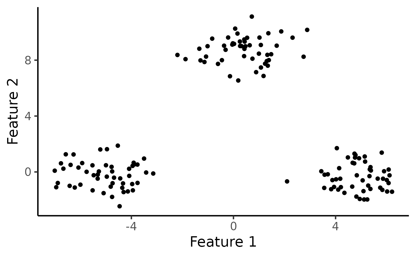
# Visualize the data
ggplot(data.frame(X), aes(x=X1, y=X2)) +
geom_point(cex=2) + xlab("Feature 1") + ylab("Feature 2") +
 theme_classic(base_size=18) + theme(legend.position="none") +
 scale_colour_manual(values=c("dodgerblue3", "rosybrown", "orange")) +
 theme(legend.title = element_blank(),
 plot.title = element_text(hjust = 0.5))

 k <- 3
 # Run k-means clustering with K=3
 estimated_clusters <- kmeans_estimation(X, k,iter.max = 20,seed = 2021)$final_cluster
 table(true_clusters,estimated_clusters)
#>              estimated_clusters
#> true_clusters  1  2  3
#>             1  0 50  0
#>             2  0  0 50
#>             3 50  0  0
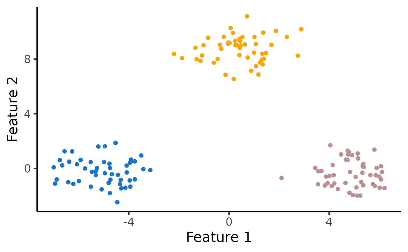
 # Visualize the clusters
 ggplot(data.frame(X), aes(x=X1, y=X2, col=as.factor(estimated_clusters))) +
 geom_point(cex=2) + xlab("Feature 1") + ylab("Feature 2") +
 theme_classic(base_size=18) + theme(legend.position="none") +
 scale_colour_manual(values=c("dodgerblue3", "rosybrown", "orange")) +
 theme(legend.title = element_blank(), plot.title = element_text(hjust = 0.5))