Technical details

Figure 1: We simulated one dataset according to \(MN_{100\times 10}(\mu, \textbf{I}_{100}, \Sigma)\), where \(\mu_i = (1,0_9)^T\) for \(i=1,\ldots, 50\) and \(\mu_i = (0_9,1)^T\) for \(i=51,\ldots, 100\), and \(\Sigma_{ij} = 1\{i=j\}+0.4\cdot 1\{i\neq j\}\). (a): Empirical distribution of feature 2 based on the simulated data set. In this case, all observations have the same mean for feature 2. (b): We apply k-means clustering to obtain two clusters and plot the empirical distribution of feature 2 stratified by the clusters. (c): Quantile-quantile plot of naive z-test (black) our proposed p-values (orange) applied to the simulated data sets for testing the null hypotheses for a difference in means for features 2–8.

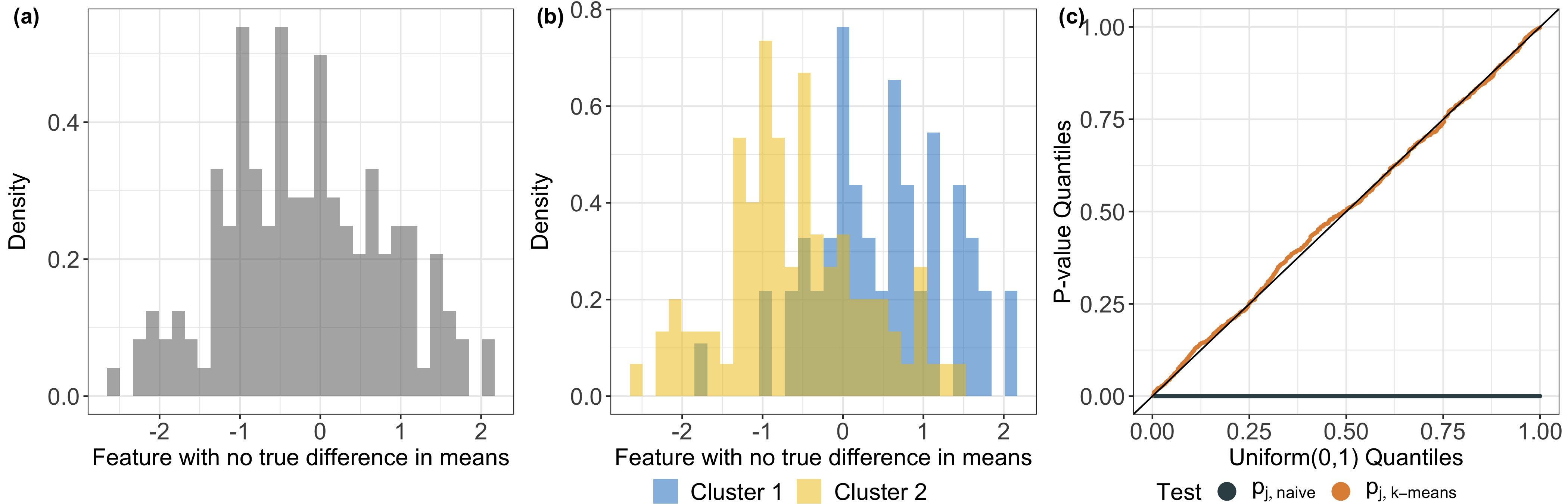
Overview

This package, as well as its underlying methodology, is motivated by the practical need to interpret and validate groups of observations obtained via clustering. In this case, a common validation approach involves testing differences in feature means between observations in two estimated clusters. However, classical hypothesis tests lead to an inflated Type I error rate, because the p-values are computed using the same set of data used for generating the hypothesis.

To overcome this problem, we propose a new test for the difference in means in a single feature between a pair of clusters obtained using hierarchical or k-means clustering. More details can be found in our manuscript (Chen and Gao, 2023+).

In this tutorial, we provide an overview of our selective inference approach. Details for the computationally-efficient implementation of our proposed p-value can be found in Sections 3 and 4 of our manuscript, available at arXiv_link_here.

Model setup

Let \(x \in \mathbb{R}^{n \times q}\) be a data matrix with \(n\) observations of \(q\) features that we want to perform clustering on. For \(\mu \in \mathbb{R}^{n \times q}\) with unknown rows \(\mu_i \in \mathbb{R}^q\) and known, positive-definite \(\Sigma \in \mathbb{R}^{q \times q}\), we assume that \(x\) is a realization of a random matrix \(X\), where rows of \(X\) are independent and drawn from a multivariate normal distribution: \[\begin{equation} X_i \sim N_q(\mu_i, \Sigma), \quad i = 1, 2, \ldots, n. \end{equation}\]

Inference for the difference in means of a single feature between two estimated clusters

Let \({C}(\cdot)\) be a clustering algorithm that takes in a data matrix \(x\) with \(n\) rows and outputs a partition of \(\{1,2, \ldots, n\}\) (e.g., hierarchical or \(k\)-means clustering). Suppose that we now want to use \(x\) to test the null hypothesis that there is no difference in the mean of the \(j\)th feature across two groups obtained by applying \({C}(\cdot)\) to \(x\), i.e., \[\begin{equation} \hat{H}_{0j}: \bar{\mu}_{\hat{G} j } = \bar{\mu}_{\hat{G}' j } \text{ versus } \hat{H}_{1j}: \bar{\mu}_{\hat{G} j } = \bar{\mu}_{\hat{G}' j }. \end{equation}\] Here, \(\hat G, \hat G' \in {C}(x)\) are a pair of estimated clusters. This is equivalent to testing \(\hat{H}_{0j}: [\mu^T \hat \nu]_j = 0\) versus \(\hat{H}_{1j}: [\mu^T \hat{\nu}]_j \neq 0\), where \(\hat{\nu\)} is the \(n\)-vector with \(i\)th element given by \[\begin{equation} [\hat{\nu}]_i = {1} \{i \in \hat{G}\}/|\hat{G}| - {1} \{i \in \hat{G}'\}/|\hat{G}'|. \end{equation}\]

This results in a challenging problem because we need to account for the clustering process that led us to test this hypothesis! Drawing from the selective inference literature, we tackle this problem by proposing the following \(p\)-value: \[\begin{align} \label{eq:selective} p_{j, \text{selective}} = \mathbb{P}_{\hat{H}_{0j}} \Big ( \big |[X^T \hat{\nu}]_j \big | \geq \big |[x^T \hat{\nu}]_j \big | ~ \Big |~ {C}(X) = {C}(x), U(X) = U(x) \Big ), \end{align}\] where \[\begin{align} U(x) = x - \frac{\hat{\nu} \Sigma_{j}^T [x^T \hat{\nu}]_j }{\|\hat{\nu}\|_2^2 \Sigma_{jj}}. \label{eq:defU} \end{align}\] In the definition of \(p_{j, \text{selective}}\), we have conditioned on (i) the estimated clusters \({C}(x)\) to account for the data-driven nature of the null hypothesis; and (ii) \(U(x)\) to eliminate the unknown nuisance parameters under the null.

We show that this \(p\)-value for testing \(\hat{H}_{0j}\) can be written as {\[\begin{align} \begin{split} \label{eq:selective_cdf} p_{j, \text{selective}} = 1 - \mathbb{F} \left (\big | [\hat{\nu}^T x]_j \big | ; 0, \Sigma_{jj}\|\hat{\nu}\|_2^2; {\hat{S}}_j \right ) + \mathbb{F}\left (-\big | [\hat{\nu}^T x]_j \big | ; 0, \Sigma_{jj} \|\hat \nu\|_2^2; {\hat{S}}_j \right ), \end{split} \end{align}\]} where \(\mathbb{F}(t; \mu, \sigma, {S})\) denotes the cumulative distribution function (CDF) of a \(N(\mu, \sigma^2)\) random variable truncated to the set \({S}\), \(x'(\phi,j) = x + (\phi - ( \bar{x}_{\hat{G}j} - \bar{x}_{\hat{G'}j})) \left ( \frac{ \hat{\nu} }{ \|\hat{\nu}\|_2^2 } \right ) \left ( \frac{\Sigma_j}{\Sigma_{jj}} \right )^T,\) and \[\begin{equation} \hat S_j = \left \{ \phi \in \mathbb{R}: C(x) = {C}\left(x'(\phi,j)\right ) \right \}. \label{eq:defS} \end{equation}\].

While the notation in the last paragraph might seem daunting, the intuition is simple: since \(p_{j, \text{selective}}\) can be rewritten into sums of CDFs of truncated univariate normal random variable evaluated at some given values, it suffices to characterize the truncation set \(\hat S_j\).

We demonstrate how to compute \(\hat S_j\) for hierarchical clustering (and a close variant of it for \(k\)-means clustering) in our manuscript, and our software implements an efficient calculation of this \(p\)-value by analytically characterizing the relevant sets. Our key insight is that the set \(\hat S_j\) can be expressed as the intersection of solutions to a series of quadratic inequalities of \(\phi\), leading to efficient and analytical characterization of the set, and consequently, the \(p\)-value. The test based on the resulting \(p\)-value will control the selective Type I error rate, in the sense of Lee et al. (2016) and Fithian et al. (2014); see also Figure 1(c) of this tutorial. Additional details can be found in Sections 3 and 4 of Chen and Gao (2023+).

Remark: by contrast, the naive \(p\)-value (used in a two-sample z-test) takes the form \[\begin{equation} p_{j, \text{naive}} = \mathbb{P}_{\hat{H}_{0j}} \left ( | [X^T \hat{\nu}^T]_j | \geq | [x^T \hat{\nu}]_j| \right ), \label{eq:naive} \end{equation}\] which ignores the fact that the contrast vector \(\nu\) is estimated from the data via clustering, and therefore leads to a test with an inflated Type I error rate.

References

Chen YT and Gao LL. (2023+) Testing for a difference in means of a single feature after clustering. arXiv preprint.

Fithian W, Sun D, Taylor J. (2014) Optimal Inference After Model Selection. arXiv:1410.2597 [mathST].

Lee J, Sun D, Sun Y, Taylor J. Exact post-selection inference, with application to the lasso. Ann Stat. 2016;44(3):907-927. doi:10.1214/15-AOS1371