Tutorials for hierarchical clustering inference
Tutorials_hier.RmdIn this tutorial, we demonstrate basic use of the CADET
package for testing for a difference in feature means between clusters
obtained via hierarchical clustering.
First we load relevant packages:
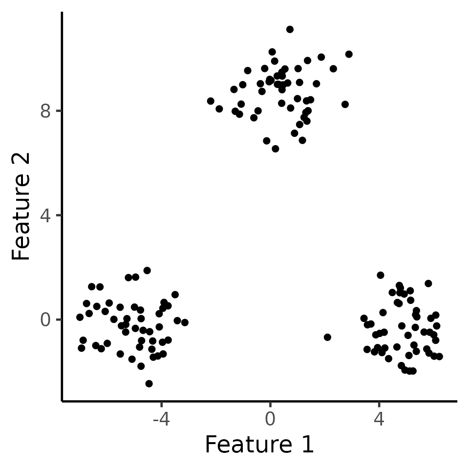
We first generate data according to \(\mathbf{X} \sim {MN}_{n\times q}(\boldsymbol{\mu}, \textbf{I}_n, \sigma^2 \textbf{I}_q)\) with \(n=150,q=2,\sigma=1,\) and \[\begin{align} \label{eq:power_model} \boldsymbol{\mu}_1 =\ldots = \boldsymbol{\mu}_{50} = \begin{bmatrix} -\delta/2 \\ 0_{q-1} \end{bmatrix}, \; {\boldsymbol\mu}_{51}=\ldots = \boldsymbol{\mu}_{100} = \begin{bmatrix} 0_{q-1} \\ \sqrt{3}\delta/2 \end{bmatrix} ,\; \boldsymbol{\mu}_{101}=\ldots = \boldsymbol{\mu}_{150} = \begin{bmatrix} \delta/2 \\ 0_{q-1} \end{bmatrix}. \end{align}\] Here, we can think of \({C}_1 = \{1,\ldots,50\},{C}_2 = \{51,\ldots,100\},{C}_3 = \{101,\ldots,150\}\) as the “true clusters”. In the figure below, we display one such simulation \(\mathbf{x}\in\mathbb{R}^{100\times 2}\) with \(\delta=10\).
set.seed(2022)
n <- 150
true_clusters <- c(rep(1, 50), rep(2, 50), rep(3, 50))
delta <- 10
q <- 2
mu <- rbind(c(delta / 2, rep(0, q - 1)), c(rep(0, q - 1), sqrt(3) * delta / 2), c(-delta / 2, rep(0, q - 1)))
sig <- 1
X <- matrix(rnorm(n * q, sd = sig), n, q) + mu[true_clusters, ]

ggplot(data.frame(X), aes(x = X1, y = X2)) +
  geom_point(cex = 2) +
  xlab("Feature 1") +
  ylab("Feature 2") +
  theme_classic(base_size = 18) +
  theme(legend.position = "none") +
  scale_colour_manual(values = c("dodgerblue3", "rosybrown", "orange")) +
  theme(
    legend.title = element_blank(),
    plot.title = element_text(hjust = 0.5)
  )
Hierarchical clustering (K=3)
In the code below, we call the hcl function in the
fastclusters package to estimate clusters using average
linkage. In the figure below, observations are colored by the clusters
obtained via cutting the dendrograms at \(K=3\).
k <- 3
hcl <- hclust(dist(X, method = "euclidean")^2, method = "average")
estimated_clusters <- cutree(hcl, 3)
ggplot(data.frame(X), aes(x = X1, y = X2, col = as.factor(estimated_clusters))) +
  geom_point(cex = 2) +
  xlab("Feature 1") +
  ylab("Feature 2") +
  theme_classic(base_size = 18) +
  theme(legend.position = "none") +
  scale_colour_manual(values = c("dodgerblue3", "rosybrown", "orange")) +
  theme(
    legend.title = element_blank(),
    plot.title = element_text(hjust = 0.5)
  )
Inference for a single feature mean after hierarchical clustering
In this section, we demonstrate how to use our software to obtain
\(p\)-values for testing for a
difference in the means of a single feature between a pair of clusters
identified via hierarchical clustering (using average linkage as an
example). As an example, consider testing for a difference in the first
feature (x axis) between the blue cluster (labeled as 1 in
estimated_clusters) and the pink cluster (labeled as 3 in
estimated_clusters).
The code below demonstrates how to use the function
test_hier_clusters_exact_1f, which performs inference on
the specified two estimated clusters. After obtaining the inferential
result, we call the summary method to get a summary of the results, in
the form of a data frame.
cluster_1 <- 1
cluster_2 <- 3
cl_inference_demo <- test_hier_clusters_exact_1f(X = X, link = "average", hcl = hcl, K = 3, k1 = cluster_1, k2 = cluster_2, feat = 1)
summary(cl_inference_demo)
#>   cluster_1 cluster_2 test_stat  p_selective      p_naive
#> 1         1         3  9.910708 2.868783e-26 4.596766e-31
In the summary, we have the empirical difference in means of the
first feature between the two clusters, i.e.,\(\sum_{i\in
{\hat{{G}}}}\mathbf{x}_{i,2}/|\hat{{G}}| - \sum_{i\in
\hat{G}'}\mathbf{x}_{i,2}/|\hat{G}'|\)
(test_stats), the naive p-value based on a z-test
(p_naive), and the selective \(p\)-value (p_selective). In
this case, the test based on \(p_{1,\text{selective}}\) can reject this
null hypothesis that the blue and pink clusters have the same mean in
the first feature (\(p_{1,\text{selective}}<0.001\)).
Inference for a single feature mean after hierarchical clustering when the null hypothesis holds
In this section, we demonstrate that our proposed \(p\)-value yields reasonable results when the null hypothesis does hold. Consider the same data and clustering assignment as before, there is no difference in means in the second feature between cluster 1 (grey cluster) and cluster 3 (blue cluster).
Now the selective \(p\)-value yields a much more moderate \(p\)-value, and the test based on it cannot reject the null hypothesis when it holds. By contrast, the naive \(p\)-value is tiny and leads to an anti-conservative test.
cluster_1 <- 1
cluster_2 <- 3
cl_inference_demo <- test_hier_clusters_exact_1f(
  X = X, link = "average",
  hcl = hcl, K = 3, k1 = cluster_1, k2 = cluster_2, feat = 2
)
summary(cl_inference_demo)
#>   cluster_1 cluster_2  test_stat p_selective   p_naive
#> 1         1         3 -0.1766818   0.8362984 0.8362984