Real data application

In this tutorial, we demonstrate how to apply the functions in the SpikeInference package to a calcium imaging dataset collected initially in Chen et al. (2013).

First we load the package and read in data from GitHub:

require(SpikeInference)
#> Loading required package: SpikeInference
require(RCurl)
#> Loading required package: RCurl
require(ggplot2)
#> Loading required package: ggplot2
require(latex2exp)
#> Loading required package: latex2exp
require(scales)
#> Loading required package: scales
require(dplyr)
#> Loading required package: dplyr
#> 
#> Attaching package: 'dplyr'
#> The following objects are masked from 'package:stats':
#> 
#>     filter, lag
#> The following objects are masked from 'package:base':
#> 
#>     intersect, setdiff, setequal, union
consistent_color <- scales::hue_pal()(8)


link_calcium <- getURL("https://raw.githubusercontent.com/yiqunchen/SpikeInference-experiments/main/input_files/7.train.calcium.csv")
calcium_1 <- read.csv(text = link_calcium)
link_spike <- getURL("https://raw.githubusercontent.com/yiqunchen/SpikeInference-experiments/main/input_files/7.train.spikes.csv")
spike_1 <- read.csv(text = link_spike)

We will focus on recording 27 in experiment 7 for this tutorial. We set \(\gamma=0.9857\) based on the sampling rate and the property of the calcium indicator used in the experiment.

curr_exp_num <- 7
curr_cell_num <- 29
sampling_freq <- 100
T_end = sum(!is.na(calcium_1[,curr_cell_num]))
gam_star <- 1-(1/100/0.7)

To account for the non-zero baseline in the recording, we estimate spikes using the following optimization problem with \(\lambda = 0.63\) and \(\beta_0 = -0.3\): \[\begin{equation} \text{minimize}_{c_1,...,c_T\geq 0} \left\{\frac{1}{2}\sum_{t=1}^T ( y_t - c_t + \beta_0)^2 + \lambda \sum_{t=2}^T 1(c_t \neq \gamma c_{t-1}) \right\}. \end{equation}\] These values were chosen using a two-dimensional grid-search on the values of \(\lambda\) and \(\beta_0\). A function to implement the search can be found here.

curr_lambda <- 0.6309573
beta_0_star <- -0.3
fit_spike <- spike_estimates(calcium_1[1:T_end,curr_cell_num]+beta_0_star,
                             gam_star, curr_lambda)
fit_calcium <- spike_estimates(calcium_1[1:T_end,curr_cell_num]+beta_0_star,
                               gam_star, curr_lambda)$estimated_calcium

We will use \(h=20\) and estimate variance using \(\hat{\sigma}^2 = \frac{1}{T-1}(y_t-\hat{c}_t)^2\).

h <- 20
sigma_2_hat <- var(calcium_1[1:T_end,curr_cell_num]+beta_0_star-fit_calcium)

selective_p_val <- spike_inference(dat = calcium_1[1:T_end,curr_cell_num]+beta_0_star, 
                                   decay_rate = gam_star,
                                   tuning_parameter = curr_lambda, 
                                   window_size = h,
                                   sig2 = sigma_2_hat, 
                                   return_ci=FALSE)

Some data wrangling to get our result ready for plotting.

current_cell <- data.frame(calcium = calcium_1[1:T_end,curr_cell_num]+beta_0_star, 
                           spike = spike_1[1:T_end,curr_cell_num],
                           fit_calcium=fit_calcium) 
current_cell <- current_cell %>% 
  mutate(cam_time = 1/100*c(1:nrow(current_cell)), no_prune_time = 0) 
current_cell[fit_spike$spikes,'no_prune_time'] <- 1

current_cell$selective_p_val <- NA
current_cell[selective_p_val$spikes,'selective_p_val'] <- selective_p_val$pvals

We will present our plots in three successive zoom levels. In all figures below, the cell’s fluorescence trace is displayed in gray; spikes estimated via the \(\ell_0\) problem are displayed in orange; the spikes with selective \(p\)-values below \(0.05\) (with \(h=20\)) are displayed in blue; and the true spike times are shown in black.

Zoom level 1; entire recording: 240 seconds

current_cell %>%
  ggplot(aes(x=cam_time,y=calcium))+
  geom_point(color = "grey", size = 0.6, alpha = 0.8)+
  #geom_line(color="blue",aes(x=cam_time,y=fit_calcium))+
  xlab("Time (seconds)") +
  ylab("Fluorescence")+
  coord_cartesian(ylim=c(-4, max(current_cell %>% select(calcium) * 1.001)))+
  theme_bw() + 
  theme(panel.border = element_blank(), panel.grid.major = element_blank(),
        panel.grid.minor = element_blank(), axis.line = element_line(colour = "black"))+
  geom_segment(data =  current_cell%>%
                 filter(no_prune_time==1)%>%
                 select(cam_time), 
               aes(x = cam_time, xend = cam_time,
                   y = -0.5, yend = -1.5, color = "orange"),
               alpha = 0.75)+
  geom_segment(data =  current_cell %>%
                 filter((no_prune_time==1)&!is.na(selective_p_val)&(selective_p_val<=0.05))%>%
                 select(cam_time), 
               aes(x = cam_time, xend = cam_time,
                   y = -2.0, yend = -3.0,color = "royalblue"),
               alpha = 0.75)+
  geom_segment(data = current_cell%>%
                 filter(spike>0)%>%
                 select(cam_time), 
               aes(x = cam_time, xend = cam_time,
                   y = -3.5, yend = -4.5, color = "black"),
               alpha = 0.75) +
  scale_colour_manual(name = unname(TeX(c(""))),
                      values =  c("orange","royalblue","black"),
                      breaks = c("orange", "royalblue","black"),
                      labels = unname(TeX(c("l_0 solution",
                                            "l_0 solution, $p<0.05$, h=20",
                                            "True spikes"))))+
  guides(colour = guide_legend(override.aes = list(size = 15)))+
  theme(legend.position="bottom",
        legend.text=element_text(size=15),
        axis.title=element_text(size=15),
        axis.text = element_text(size=15))+
  scale_x_continuous(breaks = scales::pretty_breaks(n = 10))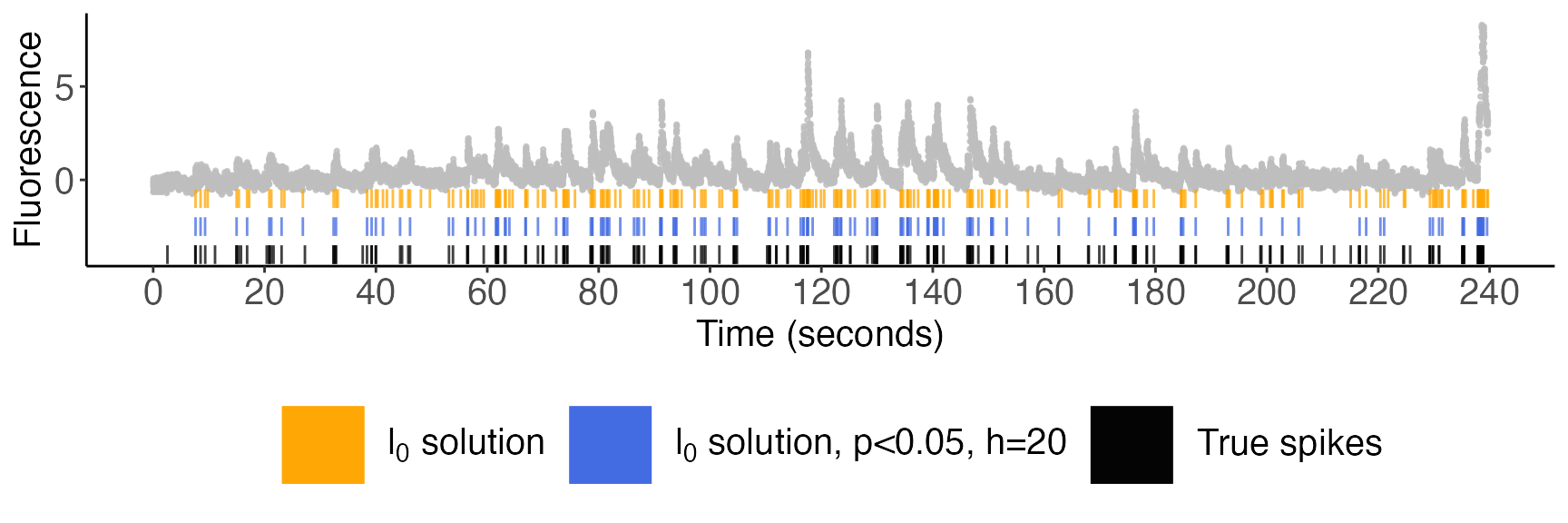

Zoom level 2; 50-100 seconds

current_cell %>%
  filter(cam_time>=50,cam_time<=100) %>%
  ggplot(aes(x=cam_time,y=calcium))+
  geom_point(color = "grey", size = 0.6, alpha = 0.8)+
  xlab("Time (seconds)") +
  ylab("Fluorescence")+
  coord_cartesian(ylim=c(-4, max(current_cell %>%
                                   filter(cam_time>=50,cam_time<=100)%>%
                                   pull(calcium)) * 1.001))+
  theme_bw() + 
  theme(panel.border = element_blank(), panel.grid.major = element_blank(),
        panel.grid.minor = element_blank(), 
        axis.line = element_line(colour = "black"))+
  geom_segment(data =  current_cell%>%
                 filter(no_prune_time==1)%>%
                 filter(cam_time>=50,cam_time<=100) %>%
                 select(cam_time), 
               aes(x = cam_time, xend = cam_time,
                   y = -0.5, yend = -1.5, color = "orange"),
               alpha = 0.75)+
  geom_segment(data =  current_cell%>%
                 filter(cam_time>=50,cam_time<=100) %>%
                 filter((no_prune_time==1)&!is.na(selective_p_val)&(selective_p_val<=0.05))%>%
                 select(cam_time), 
               aes(x = cam_time, xend = cam_time,
                   y = -2.0, yend = -3.0,color = "royalblue"),
               alpha = 0.75)+
  geom_segment(data = current_cell%>%
                 filter(cam_time>=50,cam_time<=100) %>%
                 filter(spike>0)%>%
                 select(cam_time), 
               aes(x = cam_time, xend = cam_time,
                   y = -3.5, yend = -4.5, color = "black"),
               alpha = 0.75) +
  scale_colour_manual(name = unname(TeX(c(""))),
                      values =  c("orange","royalblue","black"),
                      breaks = c("orange", "royalblue","black"),
                      labels = unname(TeX(c("l_0 solution",
                                            "l_0 solution, $p<0.05$, h=20",
                                            "True spikes"))))+
  guides(colour = guide_legend(override.aes = list(size = 15)))+
  theme(legend.position="bottom",
        legend.text=element_text(size=15),
        axis.title=element_text(size=15),
        axis.text = element_text(size=15))+
  scale_x_continuous(breaks = scales::pretty_breaks(n = 15))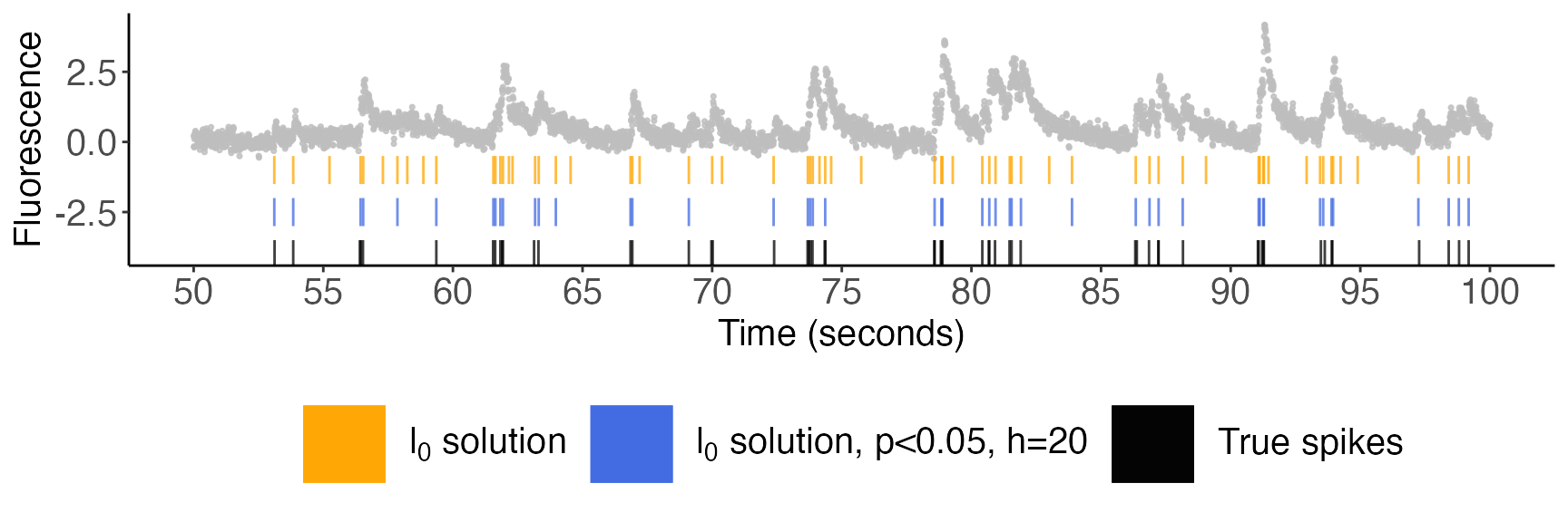

Zoom level 3; 75-90 seconds

current_cell %>%
  filter(cam_time>=75,cam_time<=90) %>%
  ggplot(aes(x=cam_time,y=calcium))+
  geom_point(color = "grey", size = 0.6, alpha = 0.8)+
  xlab("Time (seconds)") +
  ylab("Fluorescence")+
  coord_cartesian(ylim=c(-4, max(current_cell%>%
                                   filter(cam_time>=75,cam_time<=90) %>%select(calcium) * 1.001)))+
  theme_bw() + 
  theme(panel.border = element_blank(), panel.grid.major = element_blank(),
        panel.grid.minor = element_blank(), axis.line = element_line(colour = "black"))+
  geom_segment(data =  current_cell%>%
                 filter(no_prune_time==1)%>%
                 filter(cam_time>=75,cam_time<=90) %>%
                 select(cam_time), 
               aes(x = cam_time, xend = cam_time,
                   y = -0.5, yend = -1.5, color = "orange"),
               alpha = 0.75)+
  geom_segment(data =  current_cell%>%
                 filter(cam_time>=75,cam_time<=90) %>%
                 filter((no_prune_time==1)&!is.na(selective_p_val)&(selective_p_val<=0.05))%>%
                 select(cam_time), 
               aes(x = cam_time, xend = cam_time,
                   y = -2.0, yend = -3.0,color = "royalblue"),
               alpha = 0.75)+
  geom_segment(data = current_cell%>%
                 filter(cam_time>=75,cam_time<=90) %>%
                 filter(spike>0)%>%
                 select(cam_time), 
               aes(x = cam_time, xend = cam_time,
                   y = -3.5, yend = -4.5, color = "black"),
               alpha = 0.75) +
  scale_colour_manual(name = unname(TeX(c(""))),
                      values =  c("orange","royalblue","black"),
                      breaks = c("orange", "royalblue","black"),
                      labels = unname(TeX(c("l_0 solution",
                                            "l_0 solution, $p<0.05$, h=20",
                                            "True spikes"))))+
  guides(colour = guide_legend(override.aes = list(size = 15)))+
  theme(legend.position="bottom",
        legend.text=element_text(size=15),
        axis.title=element_text(size=15),
        axis.text = element_text(size=15))+
  scale_x_continuous(breaks = scales::pretty_breaks(n = 15))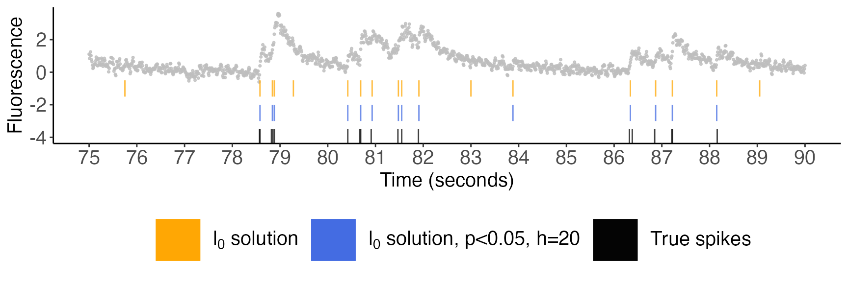

We see that the estimated spikes with p-values less than 0.05 match very closely with the true spikes. For example, the \(\ell_0\) optimization problem estimates spikes near 75.8, 79.3, 83.0, and 89.1 seconds. None of these correspond to a true spike, and none have a p-value less than 0.05. Thus, the spikes with p-values above 0.05 appear to be false positives. By contrast, those with p-values below 0.05 are mostly true positives.

References

Chen T-W, Wardill TJ, Sun Y, Pulver SR, Renninger SL, Baohan A, Schreiter ER, Kerr RA, Orger MB, Jayaraman V, Looger LL, Svoboda K, Kim DS. Ultrasensitive fluorescent proteins for imaging neuronal activity. Nature. 2013;499(7458):295-300. doi:10.1038/nature12354

Chen YT, Jewell SW, Witten DM. (2021) Quantifying uncertainty in spikes estimated from calcium imaging data. arXiv:2103.0781 [statME].