Technical details
technical_details.Rmd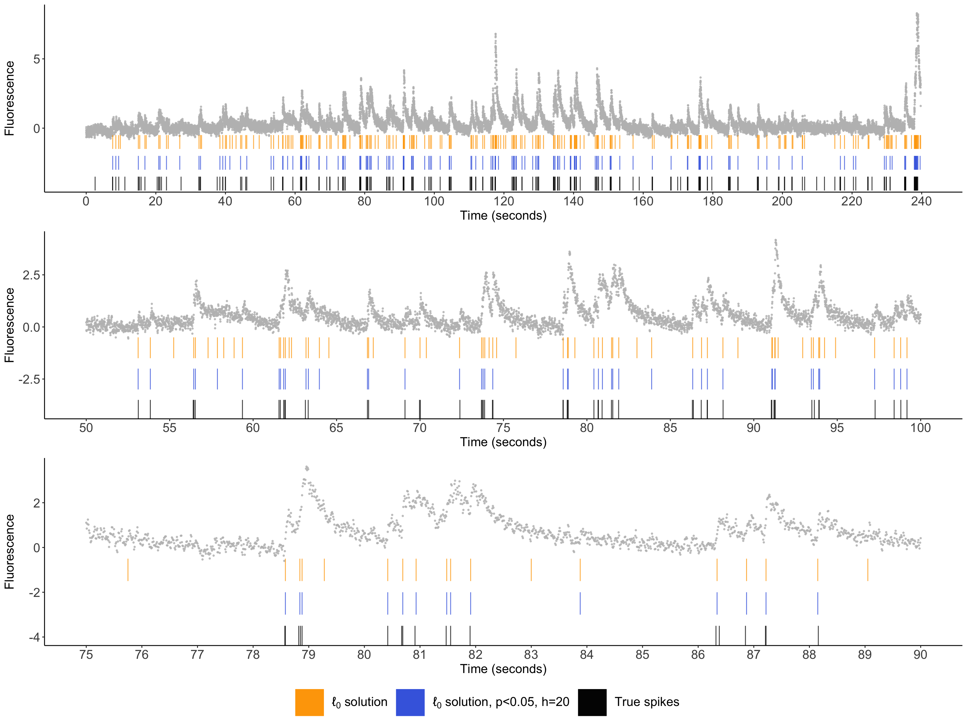
Figure 1: Illustrative example for recording 29 from Chen et al. (2013), which uses the GCaMP6f indicator. The cell’s fluorescence trace is displayed in gray. Spikes estimated via the \(\ell_0\) problem are displayed in orange; the spikes with selective \(p\)-values below \(0.05\) (with \(h=20\)) are displayed in blue; and the true spike times are shown in black.
Overview
Calcium imaging is an increasingly popular technique in neuroscience for recording the activity of large populations of neurons in vivo. When a neuron spikes, calcium floods the cell. Due to the use of fluorescent calcium indicators, this leads to a rapid increase in calcium. Therefore, for each neuron, calcium imaging results in a time series of fluorescence intensities that can be seen as a first-order approximation to its unobserved spike times. As an example, we plot one such recording in grey (see Figure 1). Typically, the scientific interest lies in the unobserved spike times, rather than the observed fluorescence traces.
After we estimated spikes from the calcium imaging data, it’s natural to want to test whether the estimated spikes correspond to a true increase in calcium. However, a naive approach that doesn’t account for the fact that the spikes are estimated from the same data used for testing will lead to inflated selective Type I error — that is, the probability of falsely rejecting the null hypothesis, given that we decided to conduct the test.
To tackle this problem, we propose a selective inference framework to compute valid \(p\)-values for hypotheses involving the estimated spikes. In a nutshell, we compute the probability of observing such a large increase in fluorescence under the null hypothesis, given that we estimated a spike at this position. In addition, we develop a computationally-efficient implementation of this framework in the case of the \(\ell_0\) spike detection algorithm.
In this tutorial, we illustrate a test of the null hypothesis that the calcium is decaying exponentially (i.e., there are no true spikes) near spikes estimated via an \(\ell_0\) penalized problem. Details for our method can be found in our manuscript at https://arxiv.org/abs/2103.07818.
Model setup
We consider the AR(1) generative model \[Y_t = c_t + \epsilon_t, \epsilon_t \sim N(0, \sigma^2), \; t = 1,\ldots, T,\] where \[c_t = \gamma c_{t-1} + z_t, z_t\geq 0, \; t = 2,\ldots, T.\] In words, this says that when \(z_t=0\), calcium decays exponentially at a (known) rate \(\gamma\in(0,1)\). If \(z_t>0\), then there is a spike at the \(t\)th timestep. We denote the locations of true spikes, \(\{t:z_t> 0\}\), as \(\{\tau_1,\ldots, \tau_K\}\). Without loss of generality, we assume that \(\tau_1 < \ldots < \tau_K\), and we use the convention that \(\tau_0 =0\) and \(\tau_{K+1} = T\).
\(\ell_0\) spike estimation
We estimate spikes based on noisy observations \(y_t, t = 1, \ldots, T\) by solving the \(\ell_0\) penalized optimization problem: \[\begin{equation} \text{minimize}_{c_1,...,c_T\geq 0} \left\{\frac{1}{2}\sum_{t=1}^T ( y_t - c_t )^2 + \lambda \sum_{t=2}^T 1(c_t \neq \gamma c_t-1) \right\}. \label{eq:ell_0} \end{equation}\]
Estimated spikes correspond to the timepoints at which the estimated calcium \(\hat{c}_t\) does not decay exponentially, i.e., \(\{\hat{\tau}_1,\ldots,\hat{\tau}_{\hat{K}}\} = \{t: \hat{c}_{t+1} -\gamma \hat{c}_{t} \neq 0\}\), where \(\hat{K}\) is the number of estimated spikes. Moreover, in practice, we are only interested in estimated spikes associated with an increase (as opposed to a decrease) in estimated calcium.
Inference for the presence of spikes
To quantify the uncertainty of these estimates, we test the null hypothesis that the calcium in the neighborhood of an estimated spikes decays exponentially. In particular, consider the \(j\)th estimated spike location, denoted as \(\hat\tau_j\), under a simple assumption that there are no spikes within a window of \(+h\) and \(-h\) of \(\hat\tau_j\). Then we wish to test the null hypothesis \[\begin{equation} H_0: \nu^\top c=0 \mbox{ versus } H_1: \nu^\top c > 0, \label{eq:null-nu} \end{equation}\] where \[\nu_{t} = \begin{cases} - \frac{\gamma (\gamma^2-1)}{\gamma^2-\gamma^{-2h+2}} \gamma^{t-\hat\tau_j} , & \hat\tau_j-h+1 \leq t \leq \hat\tau_j, \\ \frac{\gamma^2 -1 }{\gamma^{2h}-1} \gamma^{t-(\hat\tau_j+1)} , & \hat\tau_j + 1\leq t \leq \hat\tau_j+h,\\ 0, & \text{ otherwise. } \\ \end{cases}\]
In a nutshell, the definition of \(\nu\) above accounts for the underlying AR(1) mean structure of \(c_t\). More intuition can be found in Section 2.1 of our manuscript (Chen et al. 2021). Intuitively, larger values of \(h\) corresponds to more data used to test the null hypothesis of interest, resulting in larger power. However, when \(h\) is larger, \(H_0\) is also less likely to hold for the same estimated spike location \(\hat\tau_j\).
Now suppose that we test for the presence of a spike only at timepoints at a given timepoint if
- we estimate a spike, and
- there is an increase in fluorescence at that timepoint.
This results in a challenging selective inference problem: we need to account for the process that led us to estimate a spike this timepoint!
This motivates the following \(p\)-value: \[\mathbb{P}_{H_0}\left(\nu^{\top} Y \geq \nu^{\top} y \;\middle\vert\; \hat\tau_j \in \mathcal{M}(Y) , \nu^{\top}Y > 0, \Pi_{\nu}^{\perp} Y= \Pi_{\nu}^{\perp} \right),\] where \(\mathcal{M}(y)\) denotes the set of spikes estimated from \(y\) via the \(\ell_0\) problem; and \(\Pi_{\nu}^{\perp}\) is an orthogonal projection operator used to eliminate nuisance parameters. We show that this \(p\)-value for testing \(H_0\) can be written as \[\mathbb{P}\left(\phi \geq \nu^\top y \; \middle|\; \hat{\tau}_j \in \mathcal{M}(y'(\phi)), \phi\geq 0\right),\] where \(\phi\sim \mathcal{N}(0,\sigma^2||\nu||_2^2)\), and \[y'(\phi) = \Pi_{\nu}^{\perp}y+\phi\cdot \frac{\nu}{||\nu||_2^2} = y+\left(\frac{\phi-\nu^{\top}y}{||\nu||_2^2}\right)\nu\] is a perturbation of the observed data \(y\), along the direction of \(\nu\).
Moreover, if we denote \(\mathcal{S}=\{\phi: \hat\tau_j \in \mathcal{M}(y'(\phi))\}\), the \(p\)-value can be equivalently expressed as \[\mathbb{P}\left(\phi \geq \nu^\top y \;\middle |\; \phi \in \mathcal{S}\cap(0,\infty)\right).\] Now since \(\phi\sim \mathcal{N}(0,\sigma^2||\nu||_2^2)\), it follows that \(\phi \;|\; \phi \in \mathcal{S}\cap(0,\infty))\) will follow a truncated normal distribution. Thus the computation of the \(p\)-value boils down to characterizing the set \(\mathcal{S}\).
Our software implements an efficient calculation of this \(p\)-value by analytically characterizing the set \(\mathcal{S}\). The resulting \(p\)-value will control the selective Type I error, in the sense of Lee et al. (2016) and Fithian et al. (2014). Additional details can be found in Sections 2 and 3 of our paper (Chen et al. 2021)).
Remark: by contrast, a naive (Wald) \(p\)-value takes the form \[\mathbb{P}\left(\phi \geq \nu^\top y \right).\] This approach will not control the selective Type I error, i.e., it will reject \(H_0\) too often when we test \(H_0\) for spikes estimated from the data.
Extensions
Our software also allows for the following extensions:
- Generate \((1-\alpha)\) selective confidence intervals for the parameter \(\nu^\top c\), the change in calcium associated with an estimated spike.
References
Chen T-W, Wardill TJ, Sun Y, Pulver SR, Renninger SL, Baohan A, Schreiter ER, Kerr RA, Orger MB, Jayaraman V, Looger LL, Svoboda K, Kim DS. Ultrasensitive fluorescent proteins for imaging neuronal activity. Nature. 2013;499(7458):295-300. doi:10.1038/nature12354
Chen YT, Jewell SW, Witten DM. (2021) Quantifying uncertainty in spikes estimated from calcium imaging data. arXiv:2103.0781 [statME].
Lee JD, Sun DL, Sun Y, Taylor JE. Exact post-selection inference, with application to the lasso. Ann Stat. 2016;44(3):907-927. doi:10.1214/15-AOS1371
Fithian W, Sun D, Taylor J. (2014) Optimal Inference After Model Selection. arXiv:1410.2597 [mathST].