Estimate spikes with an L0 penalty
spike_estimates.RdEstimate spikes with an L0 penalty
spike_estimates(
  dat,
  decay_rate,
  tuning_parameter,
  functional_pruning_out = FALSE
)
Arguments
| dat | Numeric vector; observed data. |
|---|---|
| decay_rate | Numeric; specified AR(1) decay rate \(\gamma\), a number between 0 and 1 (non-inclusive). |
| tuning_parameter | Numeric; tuning parameter \(\lambda\) for L0 spike estimation, a non-negative number. |
| functional_pruning_out | Logical; if TRUE, return cost functions for L0 spike estimation. Defaults to FALSE. |
Value
For L0 spike estimation, returns a list with elements:
estimated_calciumEstimated calcium levelsspikesThe set of estimated spikescostThe cost at each time pointn_intervalsThe number of piecewise quadratics used at each pointpiecewise_square_lossesA data frame of optimal cost functions Cost_s*(mu) for s = 1,..., T.
Details
Estimation: This function estimates spikes via an L0 penalty based on the following optimization problem: $$minimize_{c_1,...,c_T\geq 0} \frac{1}{2} \sum_{t=1}^T ( y_t - c_t )^2 + \lambda \sum_{t=2}^{T} 1(c_t \neq \gamma c_t-1) ,$$ where \(y_t\) is the observed fluorescence at the t-th timestep.
References
Jewell, S. W., Hocking, T. D., Fearnhead, P., & Witten, D. M. (2019). Fast nonconvex deconvolution of calcium imaging data. Biostatistics.
Maidstone, R., Hocking, T., Rigaill, G., & Fearnhead, P. (2017). On optimal multiple changepoint algorithms for large data. Statistics and Computing, 27(2), 519-533.
Rigaill, G. (2015). A pruned dynamic programming algorithm to recover the best segmentations with 1 to K_max change-points. Journal de la Societe Francaise de Statistique, 156(4), 180-205.
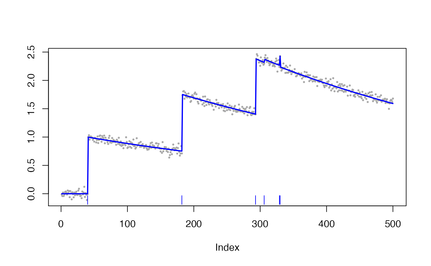
Examples
### Generate sample data sim <- simulate_ar1(n = 500, gam = 0.998, poisMean = 0.01, sd = 0.05, seed = 1) ### Fit the spike fit_spike <- spike_estimates(sim$fl, decay_rate = 0.998, tuning_parameter = 0.01) ### Plot estimated spikes plot(fit_spike)