Tutorial: k-means clustering • selectiveHotelling

library(selectiveHotelling)

Simulated data

We generate $n = 150$ observations in $p = 2$ dimensions from three groups of $50$ , whose means differ by $6$ along the first feature. The two features are correlated, and the analysis below never uses their covariance matrix.

set.seed(123)
n_per <- 50
Sigma <- matrix(c(1, 0.6, 0.6, 1), 2, 2)
noise <- matrix(rnorm(3 * n_per * 2), ncol = 2) %*% chol(Sigma)
mu <- rbind(c(-6, 0), c(0, 0), c(6, 0))[rep(1:3, each = n_per), ]
X <- mu + noise
true_group <- rep(1:3, each = n_per)

Cluster and test

selective_hotelling_test() runs $k$ -means with $K$ clusters and tests the null hypothesis that clusters k1 and k2 share one mean. It returns the selective $p$ -value and the clustering that was tested.

set.seed(1)   # fixes the random initial centers of k-means
res12 <- selective_hotelling_test(X, k1 = 1, k2 = 2, K = 3, M = 1000)
res12
#> Selective Hotelling T^2 test (unknown covariance)
#>   Clusters tested : 1 vs 2 (of K = 3)
#>   Sampler         : besag-clifford
#>   Conditioning    : pair-preserved
#>   Observed T^2    :  1195
#>   Selective p-val : 0.004965 (MC s.e. ~ 0.002)

The default path length is M = 5000; we use M = 1000 in this tutorial so that it runs quickly; the technical details explain this choice. The estimated clusters agree with the true groups:

table(cluster = res12$cluster, true_group)
#>        true_group
#> cluster  1  2  3
#>       1  0 50  0
#>       2  0  0 50
#>       3 50  0  0

cols <- c("#0072B2", "#E69F00", "#009E73")   # color-blind-safe palette
plot(X, col = cols[res12$cluster], pch = 19, xlab = "Feature 1", ylab = "Feature 2",
     main = "")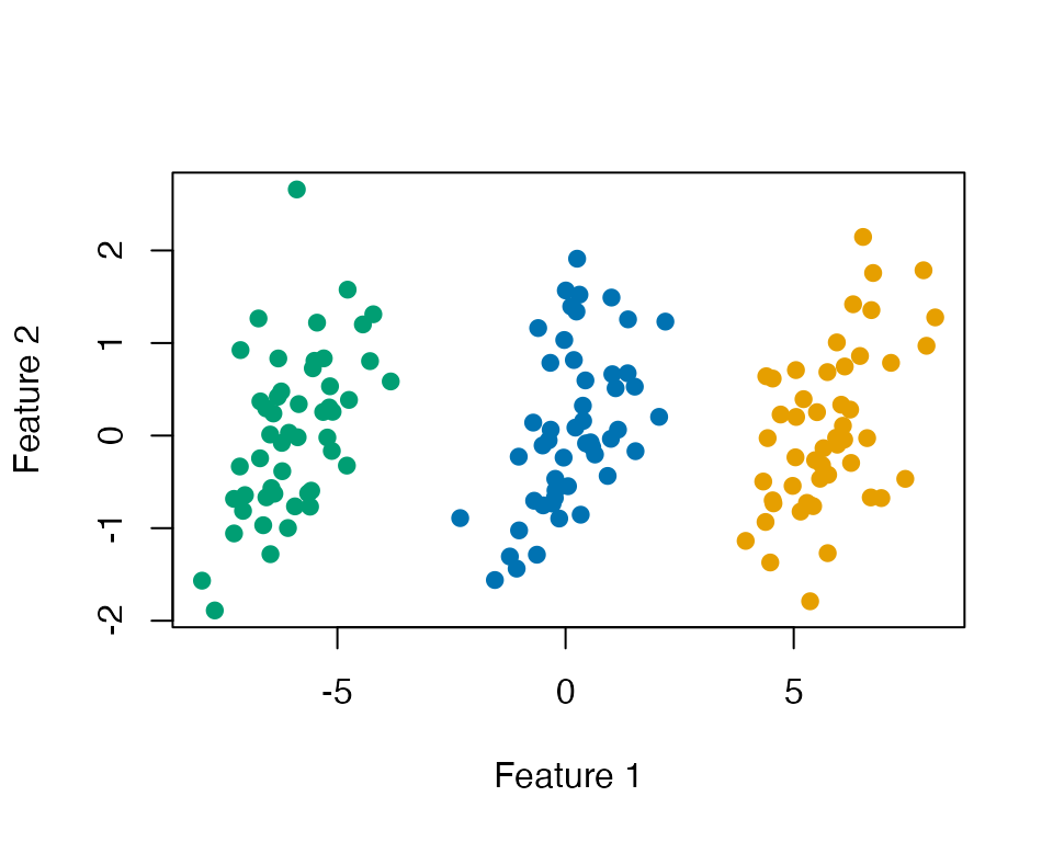

Compare with the naive test

The naive test applies Hotelling’s $T^2$ test to the estimated clusters as if they had been chosen in advance. We compute it for every pair of clusters, next to the selective test.

naive_pval <- function(X, cl, k1, k2) {
  n1 <- sum(cl == k1); n2 <- sum(cl == k2); p <- ncol(X); r <- n1 + n2
  F_stat <- (r - p - 1) / ((r - 2) * p) * hotelling_T2(X, cl, k1, k2)
  pf(F_stat, p, r - p - 1, lower.tail = FALSE)
}

pairs <- rbind(c(1, 2), c(1, 3), c(2, 3))
results <- t(apply(pairs, 1, function(k) {
  set.seed(1)   # the same initial centers, so the same clustering, for every pair
  sel <- selective_hotelling_test(X, k[1], k[2], K = 3, M = 1000)
  c(k1 = k[1], k2 = k[2], naive = naive_pval(X, sel$cluster, k[1], k[2]),
    selective = sel$pval)
}))
signif(results, 3)
#>      k1 k2    naive selective
#> [1,]  1  2 4.64e-55   0.00497
#> [2,]  1  3 8.41e-60   0.00596
#> [3,]  2  3 1.24e-84   0.00397

Both tests reject every null hypothesis here, because the three groups really differ. The difference between the tests appears when there are no groups at all.

Data with no groups

Now all $n = 150$ observations come from one Gaussian distribution, so every null hypothesis is true.

set.seed(321)
X0 <- matrix(rnorm(150 * 2), ncol = 2) %*% chol(Sigma)
res0 <- selective_hotelling_test(X0, k1 = 1, k2 = 2, K = 3, M = 1000)
c(naive = naive_pval(X0, res0$cluster, 1, 2), selective = res0$pval)
#>        naive    selective 
#> 2.023292e-26 3.001798e-01

The naive $p$ -value is tiny, although the clusters are only an artifact of $k$ -means. The selective $p$ -value is not.

Repeating the experiment

To see that this is not a coincidence, we repeat the null experiment $300$ times with $n = 60$ and plot the quantiles of the $p$ -values against those of the uniform distribution. We skip the rare data sets in which a tested cluster has fewer than three observations, for which Hotelling’s $T^2$ is not defined. A test that controls the Type I error has $p$ -values on or above the diagonal.

set.seed(2024)
sim <- t(replicate(300, {
  Xs <- matrix(rnorm(60 * 2), ncol = 2) %*% chol(Sigma)
  rs <- tryCatch(selective_hotelling_test(Xs, k1 = 1, k2 = 2, K = 3, M = 200),
                 error = function(e) NULL)   # skip the rare data sets with a tiny cluster
  if (is.null(rs)) c(naive = NA, selective = NA)
  else c(naive = naive_pval(Xs, rs$cluster, 1, 2), selective = rs$pval)
}))
sim <- sim[complete.cases(sim), ]
nrow(sim)
#> [1] 299
u <- ppoints(nrow(sim))
plot(u, sort(sim[, "naive"]), pch = 19, col = "black", xlim = c(0, 1), ylim = c(0, 1),
     xlab = "Uniform(0, 1) quantiles", ylab = "p-value quantiles")
points(u, sort(sim[, "selective"]), pch = 19, col = "steelblue")
abline(0, 1, lty = 2)
legend("topleft", c("naive", "selective"), col = c("black", "steelblue"), pch = 19,
       bty = "n")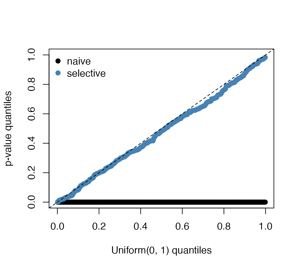

colMeans(sim <= 0.05)
#>     naive selective 
#> 1.0000000 0.0735786

At level $0.05$ , the naive test rejects 100% of these true null hypotheses and the selective test 7.4%. With about $300$ data sets, the second number has a Monte Carlo standard error of about $1.3$ percentage points; in a run with $2{,}000$ data sets, the selective test rejected $4.7\%$ .

Fixing the k-means initialization

$k$ -means depends on its random initial centers. selective_hotelling_test() draws the initial centers once, from the current random seed, and reruns $k$ -means from the same centers inside the test; set a seed before calling it to make the result reproducible. To choose the initial centers yourself, pass a clustering function to selective_hotelling_bc(), as in the tutorial for other clustering algorithms:

init <- c(1, 51, 101)                       # rows used as initial centers
cl_fun <- function(x) kmeans_with_fixed_init(x, init_centers_idx = init)$cluster
selective_hotelling_bc(X, cl_fun, k1 = 1, k2 = 2, M = 1000)$pval
#> [1] 0.006090536