Getting Started with debiasLLMReporting • debiasLLMReporting

Overview

When using LLMs as judges to evaluate other models (e.g., comparing outputs in pairwise comparisons), the LLM judge introduces measurement error. This package provides methods to correct for this bias using a small calibration sample where both human labels and LLM predictions are available.

The key insight is that with a confusion matrix estimated from calibration data, we can “debias” the prevalence estimate from the full (unlabeled) test set.

Problem Setup

Consider the task of estimating the win rate of Model A versus Model B based on pairwise comparisons. The ground truth is determined by human evaluators, but human labeling is expensive. Instead, we use an LLM judge to evaluate a large number of comparisons.

The Challenge

Let \(Y \in \{0, 1\}\) denote the true human preference (1 = Model A wins) and \(\hat{Y} \in \{0, 1\}\) denote the LLM judge’s prediction. Our goal is to estimate:

\[\theta = P(Y = 1) = \text{true win rate of Model A}\]

The naive approach is to use \(\hat{\theta}_{\text{naive}} = \frac{1}{n}\sum_{i=1}^{n} \hat{Y}_i\), but this is biased when the LLM judge makes errors.

Misclassification Model

We model the LLM judge’s errors using two parameters:

Sensitivity \(q_1 = P(\hat{Y} = 1 \mid Y = 1)\): probability the judge correctly identifies Model A wins
Specificity \(q_0 = P(\hat{Y} = 0 \mid Y = 0)\): probability the judge correctly identifies Model B wins

When \(q_0, q_1 < 1\), the naive estimator is biased. For example, if the judge has a preference for Model A (high \(q_1\), low \(q_0\)), the naive estimate will overestimate Model A’s true win rate.

The Solution: Calibration + Correction

We assume access to:

Calibration set (\(m\) samples): Both human labels \(Y\) and judge predictions \(\hat{Y}\) are observed
Test set (\(n\) samples): Only judge predictions \(\hat{Y}\) are observed

From the calibration set, we estimate \(q_0\) and \(q_1\). Then we apply correction methods to obtain an unbiased estimate of \(\theta\) with valid confidence intervals.

Setup

library(debiasLLMReporting)
set.seed(2026)

Simulated Example

Let’s simulate a scenario where:

We want to estimate the true win rate of Model A vs Model B
An LLM judge provides predictions, but with imperfect accuracy
We have a small calibration set with human labels

Generate Data

# Parameters
N <- 500          # Total samples
m <- 50           # Calibration set size (10% labeled)
theta_true <- 0.6 # True win rate for Model A
q0 <- 0.85        # Specificity: P(judge says B | human says B)
q1 <- 0.80        # Sensitivity: P(judge says A | human says A)

# Generate true labels
Y_all <- rbinom(N, 1, theta_true)

# Generate LLM judge predictions (with misclassification)
Yhat_all <- ifelse(
  Y_all == 1,
  rbinom(N, 1, q1),       # True positives detected with prob q1
  1 - rbinom(N, 1, q0)    # True negatives detected with prob q0
)

# Split into calibration and test sets
idx_cal <- sample(N, m)
idx_test <- setdiff(seq_len(N), idx_cal)

Y_cal <- Y_all[idx_cal]
Yhat_cal <- Yhat_all[idx_cal]
Yhat_test <- Yhat_all[idx_test]

Apply Estimators

# 1. Naive estimate (no correction)
naive_est <- mean(Yhat_test)
cat("Naive estimate:", round(naive_est, 3), "\n")
#> Naive estimate: 0.496

# 2. PPI (Prediction-Powered Inference)
ppi_result <- ppi_point_and_ci(
  Y_L = Y_cal,
  f_L = Yhat_cal,
  f_U = Yhat_test,
  alpha = 0.10
)

# 3. PPI++ (with optimized lambda)
ppi_pp_result <- ppi_pp_point_and_ci(
  Y_L = Y_cal,
  f_L = Yhat_cal,
  f_U = Yhat_test,
  alpha = 0.10
)

# 4. Rogan-Gladen (classical measurement error correction)
m0 <- sum(Y_cal == 0)
m1 <- sum(Y_cal == 1)
q0_hat <- mean(Yhat_cal[Y_cal == 0] == 0)
q1_hat <- mean(Yhat_cal[Y_cal == 1] == 1)
p_hat <- mean(Yhat_test)

rg_result <- rg_point_and_ci(
  p_hat = p_hat,
  q0_hat = q0_hat,
  q1_hat = q1_hat,
  n = length(Yhat_test),
  m0 = m0,
  m1 = m1,
  alpha = 0.10
)

# 5. EIF (Efficient Influence Function)
eif_result <- eif_point_and_ci(
  Y_cal = Y_cal,
  Yhat_cal = Yhat_cal,
  Yhat_test = Yhat_test,
  alpha = 0.10
)

# 6. MLE (Joint Maximum Likelihood)
mle_result <- mle_point_and_ci(
  Y_cal = Y_cal,
  Yhat_cal = Yhat_cal,
  Yhat_test = Yhat_test,
  alpha = 0.10
)

Compare Results

results <- data.frame(
  Method = c("True", "Naive", "PPI", "PPI++", "Rogan-Gladen", "EIF", "MLE"),
  Estimate = c(
    theta_true,
    naive_est,
    ppi_result$theta,
    ppi_pp_result$theta,
    rg_result$theta,
    eif_result$theta,
    mle_result$theta
  ),
  CI_Lower = c(NA, NA, ppi_result$ci_lower, ppi_pp_result$ci_lower, rg_result$ci_lower,
               eif_result$ci_lower, mle_result$ci_lower),
  CI_Upper = c(NA, NA, ppi_result$ci_upper, ppi_pp_result$ci_upper, rg_result$ci_upper,
               eif_result$ci_upper, mle_result$ci_upper)
)

results$Bias <- results$Estimate - theta_true
results$CI_Width <- results$CI_Upper - results$CI_Lower
results$Covers_True <- results$CI_Lower <= theta_true & results$CI_Upper >= theta_true

knitr::kable(results, digits = 3)

Method	Estimate	CI_Lower	CI_Upper	Bias	CI_Width	Covers_True
True	0.600	NA	NA	0.000	NA	NA
Naive	0.496	NA	NA	-0.104	NA	NA
PPI	0.576	0.486	0.661	-0.024	0.175	TRUE
PPI++	0.631	0.553	0.703	0.031	0.150	TRUE
Rogan-Gladen	0.517	0.391	0.640	-0.083	0.249	TRUE
EIF	0.620	0.522	0.710	0.020	0.188	TRUE
MLE	0.630	0.534	0.717	0.030	0.183	TRUE

Visualize

library(ggplot2)

plot_df <- results[results$Method != "True", ]
plot_df$Method <- factor(plot_df$Method,
                         levels = c("Naive", "PPI", "PPI++", "Rogan-Gladen", "EIF", "MLE"))

ggplot(plot_df, aes(x = Method, y = Estimate, color = Method)) +

  geom_point(size = 3) +
  geom_errorbar(aes(ymin = CI_Lower, ymax = CI_Upper), width = 0.2, linewidth = 1,
                na.rm = TRUE) +
  geom_hline(yintercept = theta_true, linetype = "dashed", linewidth = 1) +
  annotate("text", x = 0.6, y = theta_true + 0.03,
           label = paste("True =", theta_true), hjust = 0) +
  scale_color_manual(values = c(
    "Naive" = "#525252",
    "PPI" = "#1B9E77",
    "PPI++" = "#D95F02",
    "Rogan-Gladen" = "#7570B3",
    "EIF" = "#E6AB02",
    "MLE" = "#E7298A"
  )) +
  labs(
    title = "Win Rate Estimation with Measurement Error Correction",
    subtitle = paste0("N = ", N, ", m = ", m, " (", round(100*m/N), "% labeled)"),
    y = "Estimated Win Rate",
    x = NULL
  ) +
  theme_bw() +
  theme(legend.position = "none") +
  coord_cartesian(ylim = c(0, 1))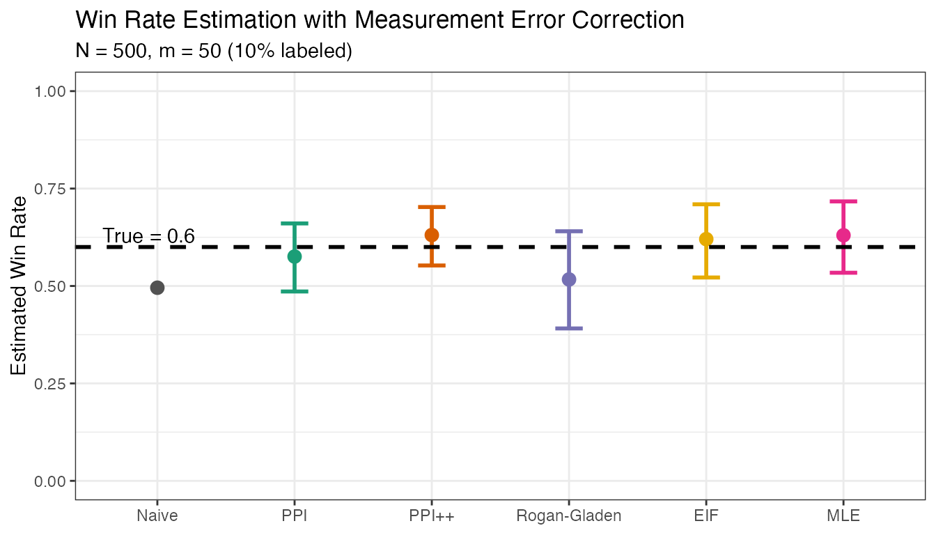

Key Takeaways

Naive estimates are biased when the LLM judge has imperfect accuracy
PPI uses the calibration residuals to correct the bias
PPI++ adaptively weights the correction to minimize variance
Rogan-Gladen uses the classical epidemiological approach based on sensitivity/specificity
EIF achieves semiparametric efficiency using the efficient influence function
MLE jointly estimates prevalence, sensitivity, and specificity via maximum likelihood

All corrected methods aim to provide valid confidence intervals with nominal coverage, while the naive estimate’s CI will not cover the true value when there’s systematic bias.

Next Steps

See the Continuous Outcomes vignette for handling continuous scores instead of binary outcomes
See the Real Data Example vignette for applying these methods to actual LLM judge evaluations