Test for a difference in means between clusters of observations identified via k-means clustering.

This function tests the null hypothesis of no difference in means between output by k-means clustering. The clusters are numbered as per the results of the kmeans_estimation function in the KmeansInference package.

kmeans_inference(
  X,
  k,
  cluster_1,
  cluster_2,
  iso = TRUE,
  sig = NULL,
  SigInv = NULL,
  iter.max = 10,
  seed = 1234,
  tol_eps = 1e-06,
  verbose = TRUE
)

Arguments

X: Numeric matrix; $n$ by $q$ matrix of observed data
k: Integer; the number of clusters for k-means clustering
cluster_1, cluster_2: Two different integers in 1,...,k; two estimated clusters to test, as indexed by the results of kmeans_estimation.
iso: Boolean. If TRUE, an isotropic covariance matrix model is used.
sig: Numeric; noise standard deviation for the observed data, a non-negative number; relevant if iso=TRUE. If it's not given as input, a median-based estimator will be by default (see Section 4.2 of our manuscript).
SigInv: Numeric matrix; if iso is FALSE, *required* $q$ by $q$ matrix specifying $\Sigma^{-1}$.
iter.max: Positive integer; the maximum number of iterations allowed in k-means clustering algorithm. Default to 10.
seed: Random seed for the initialization in k-means clustering algorithm.
tol_eps: A small number specifying the convergence criterion for k-means clustering, default to 1e-6.

Value

Returns a list with the following elements:

p_naive the naive p-value which ignores the fact that the clusters under consideration are estimated from the same data used for testing
pval the selective p-value $p_{selective}$ in Chen and Witten (2022+)
final_interval the conditioning set of Chen and Witten (2022+), stored as the Intervals class
test_stat test statistic: the difference in the empirical means of two estimated clusters
final_cluster Estimated clusters via k-means clustering

Details

For better rendering of the equations, visit https://yiqunchen.github.io/KmeansInference/reference/index.html.

Consider the generative model $X ~ MN(\mu,I_n,\sigma^2 I_q)$. First recall that k-means clustering solves the following optimization problem $$ \sum_{k=1}^K \sum_{i \in C_k} \big\Vert x_i - \sum_{i \in C_k} x_i/|C_k| \big\Vert_2^2 , $$ where $C_1,..., C_K$ forms a partition of the integers $1,..., n$, and can be regarded as the estimated clusters of the original observations. Lloyd's algorithm is an iterative apparoach to solve this optimization problem. Now suppose we want to test whether the means of two estimated clusters cluster_1 and cluster_2 are equal; or equivalently, the null hypothesis of the form $H_{0}: \mu^T \nu = 0_q$ versus $H_{1}: \mu^T \nu \neq 0_q$ for suitably chosen $\nu$ and all-zero vector $0_q$.

This function computes the following p-value: $$P \Big( || X^T\nu || \ge || x^T\nu ||_2 \; | \; \bigcap_{t=1}^{T}\bigcap_{i=1}^{n} \{ c_i^{(t)}(X) = c_i^{(t)}( x ) \}, \Pi Y = \Pi y \Big),$$ where $c_i^{(t)}$ is the is the cluster to which the $i$th observation is assigned during the $t$th iteration of the Lloyd's algorithm, and $\Pi$ is the orthogonal projection to the orthogonal complement of $\nu$. In particular, the test based on this p-value controls the selective Type I error and has substantial power. Readers can refer to the Sections 2 and 4 in Chen and Witten (2022+) for more details.

References

Chen YT, Witten DM. (2022+) Selective inference for k-means clustering. arXiv preprint. https://arxiv.org/abs/2203.15267. Lloyd, S. P. (1957, 1982). Least squares quantization in PCM. Technical Note, Bell Laboratories. Published in 1982 in IEEE Transactions on Information Theory, 28, 128–137.

Examples

library(KmeansInference)
library(ggplot2)
set.seed(2022)
n <- 150
true_clusters <- c(rep(1, 50), rep(2, 50), rep(3, 50))
delta <- 10
q <- 2
mu <- rbind(c(delta/2,rep(0,q-1)),
c(rep(0,q-1), sqrt(3)*delta/2),
c(-delta/2,rep(0,q-1)) )
sig <- 1
# Generate a matrix normal sample
X <- matrix(rnorm(n*q, sd=sig), n, q) + mu[true_clusters, ]
# Visualize the data
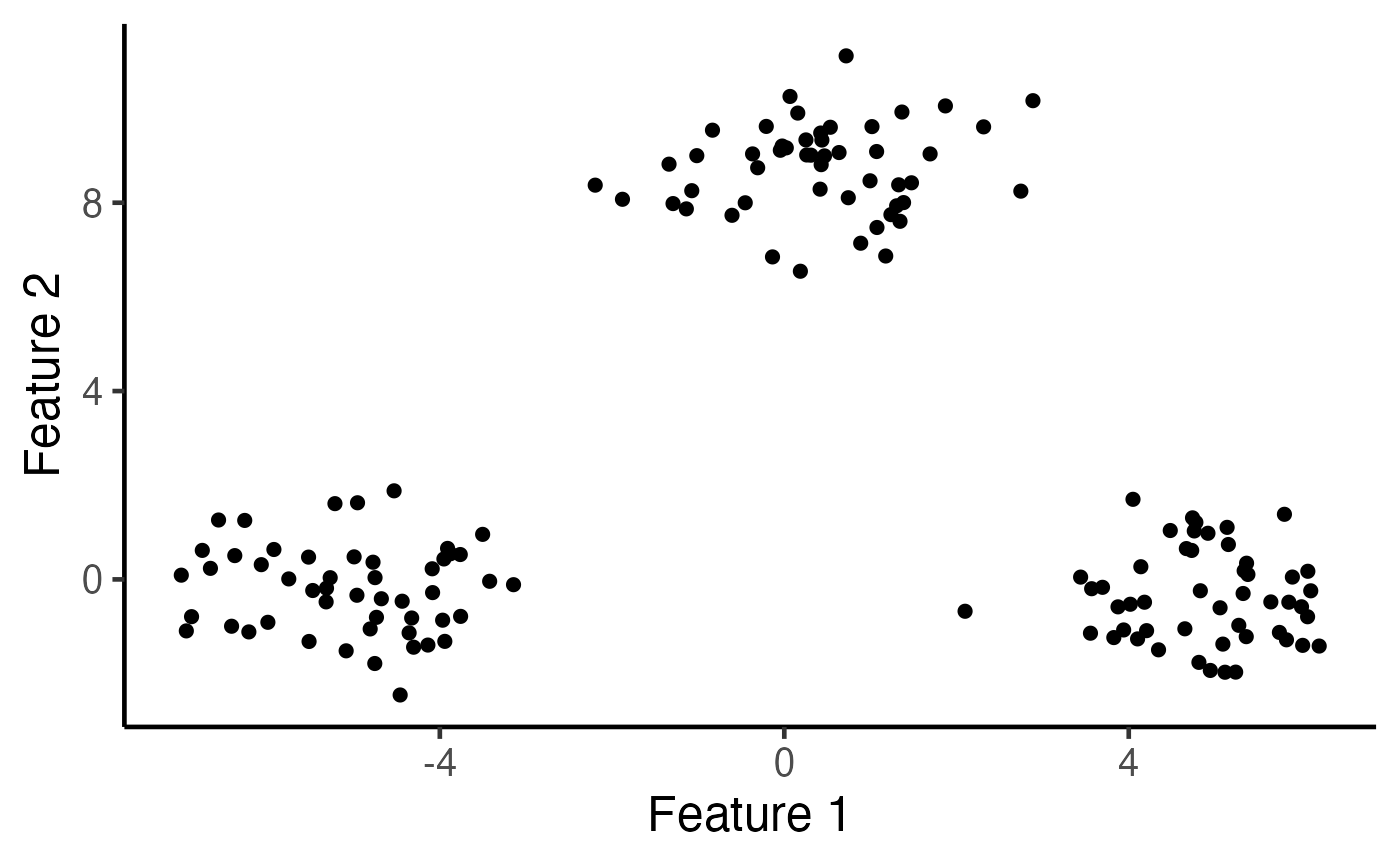
ggplot(data.frame(X), aes(x=X1, y=X2)) +
geom_point(cex=2) + xlab("Feature 1") + ylab("Feature 2") +
 theme_classic(base_size=18) + theme(legend.position="none") +
 scale_colour_manual(values=c("dodgerblue3", "rosybrown", "orange")) +
 theme(legend.title = element_blank(),
 plot.title = element_text(hjust = 0.5))

 k <- 3
 # Run k-means clustering with K=3
 estimated_clusters <- kmeans_estimation(X, k,iter.max = 20,seed = 2021)$final_cluster
 table(true_clusters,estimated_clusters)
#>              estimated_clusters
#> true_clusters  1  2  3
#>             1  0 50  0
#>             2  0  0 50
#>             3 50  0  0
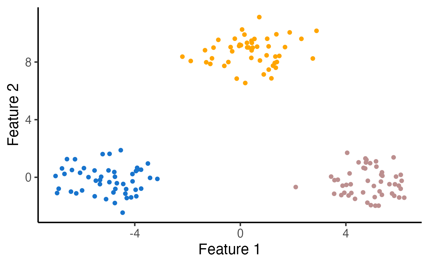
 # Visualize the clusters
 ggplot(data.frame(X), aes(x=X1, y=X2, col=as.factor(estimated_clusters))) +
 geom_point(cex=2) + xlab("Feature 1") + ylab("Feature 2") +
 theme_classic(base_size=18) + theme(legend.position="none") +
 scale_colour_manual(values=c("dodgerblue3", "rosybrown", "orange")) +
 theme(legend.title = element_blank(), plot.title = element_text(hjust = 0.5))

 ### Run a test for a difference in means between estimated clusters 1 and 3
 cluster_1 <- 1
 cluster_2 <- 3
 cl_1_2_inference_demo <- kmeans_inference(X, k=3, cluster_1, cluster_2,
 sig=sig, iter.max = 20, seed = 2021)
 summary(cl_1_2_inference_demo)
#>   cluster_1 cluster_2 test_stat  p_selective p_naive
#> 1         1         3  10.44088 4.473563e-15       0