Technical details

Figure 1: Left: One simulated dataset generated according to \(\mathcal{MN}_{100\times 2}(\textbf{0}_{100\times 2}, \textbf{I}_{100}, \sigma^2 \textbf{I}_{2})\). We apply \(k\)-means clustering to obtain three clusters. The cluster centroids are displayed as triangles. Center: Quantile-quantile plot of the Wald p-values applied to 2,000 simulated datasets from \(\mathcal{MN}_{100\times 2}(\textbf{0}_{100\times 2}, \textbf{I}_{100}, \sigma^2 \textbf{I}_{2})\). Right: Quantile-quantile plot of our proposed p-values applied to the same simulated datasets as in center.

Overview

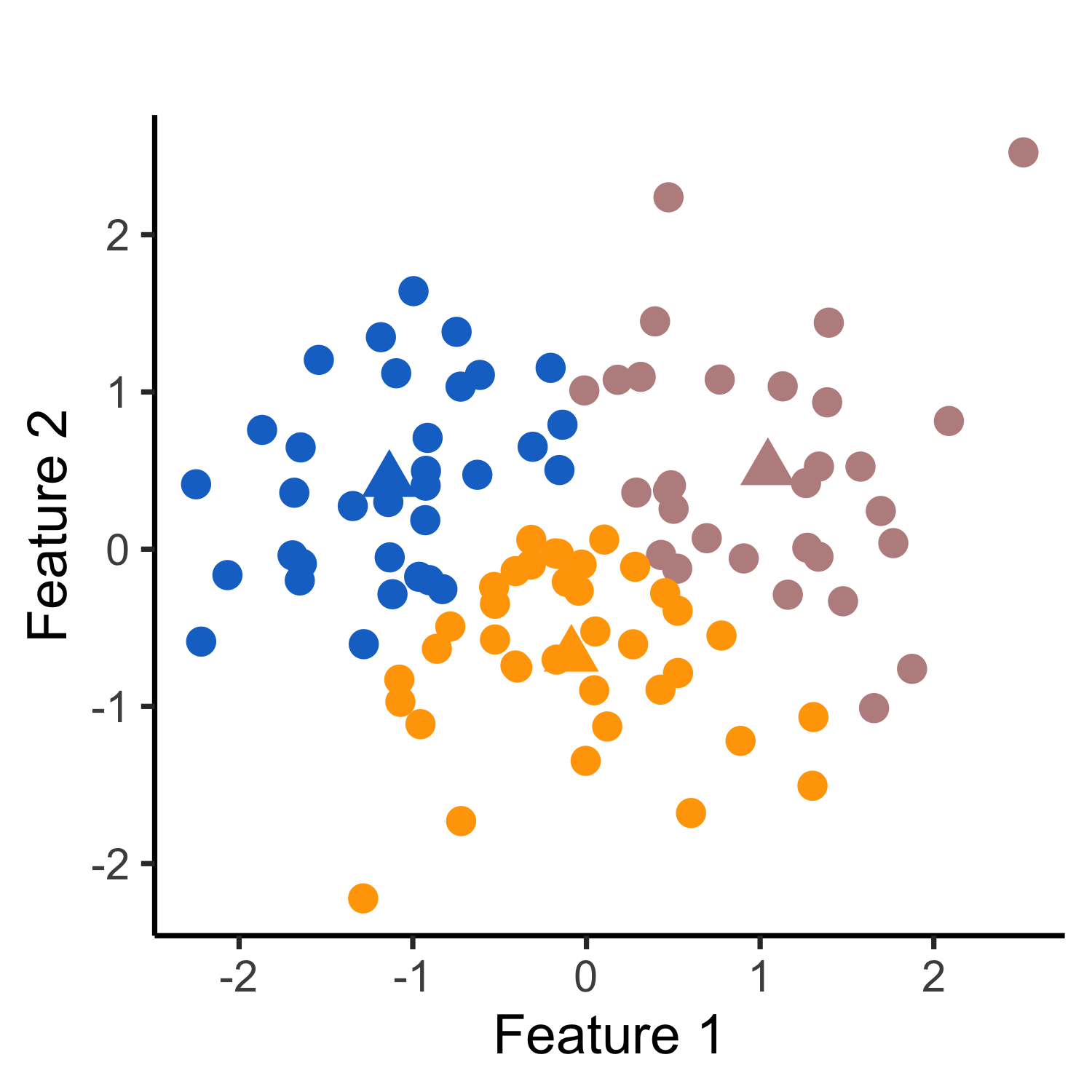
We consider the problem of testing for a difference in means between clusters of observations identified via \(k\)-means clustering, an extremely popular clustering algorithm with numerous applications. In this setting, classical hypothesis tests lead to an inflated Type I error rate, because the clusters were obtained on the same data used for testing. To overcome this problem, we propose a selective inference approach in our manuscript and describe an efficient algorithm to compute a finite-sample p-value that controls the selective Type I error for a test of the difference in means between a pair of clusters obtained using \(k\)-means clustering.

In this tutorial, we provide an overview of our selective inference approach. Details for the computationally-efficient implementation of our proposed p-value can be found in Section 3 of our manuscript, available at arXiv_link_here.

Model setup

We consider the following simple and well-studied model for \(n\) observations and \(q\) features: \[\mathbf{X} \sim \mathcal{MN}_{n\times q}(\boldsymbol{\mu}, \textbf{I}_n, \sigma^2 \textbf{I}_q),\] where \(\boldsymbol{\mu} \in \mathbb{R}^{n\times q}\) has unknown rows \(\boldsymbol{\mu}_i\), and \(\sigma^2 > 0\) is unknown. This is equivalent to positing that \(X_i\sim_{ind.} \mathcal{N}(\boldsymbol{\mu}_i,\sigma^2 \textbf{I}_q)\). In addition, we use \(\mathbf{x}\) to denote a realization of the data generating model \(\mathbf{X}\).

k-means clustering

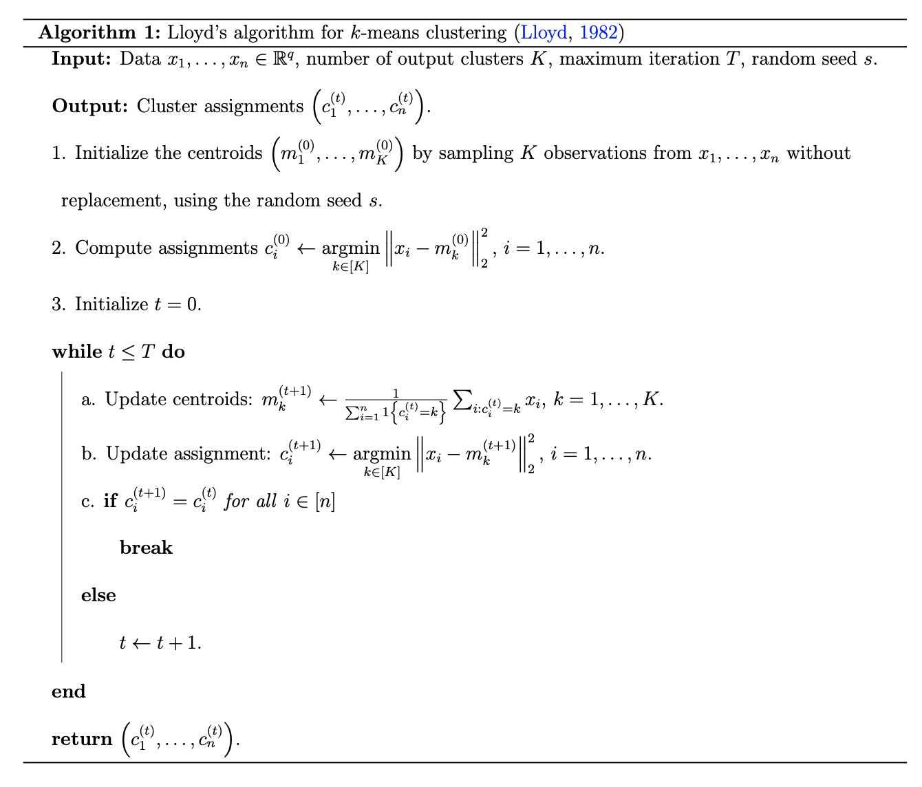
Given samples \(x_1,\ldots,x_n \in \mathbb{R}^q\), and a positive integer \(K\), \(k\)-means clustering partitions the \(n\) samples into disjoint subsets \(\hat{\mathcal{C}}_1,\ldots,\hat{\mathcal{C}}_K\) by solving the following optimization problem: \[\begin{align} &\underset{\mathcal{C}_1,\ldots,\mathcal{C}_K}{\text{minimize}}\;\left\{ \sum_{k=1}^K \sum_{i \in \mathcal{C}_k} \left\Vert x_i - \frac{\sum_{i \in \mathcal{C}_k} x_i}{|\mathcal{C}_k|} \right\Vert_2^2 \right\} \\ &\text{subject to} \; \bigcup_{k=1}^K \mathcal{C}_k = \{1,\ldots, n\},\mathcal{C}_k\cap \mathcal{C}_{k'} = \emptyset ,\forall k\neq k'. \end{align}\] It is not typically possible to solve for the global optimum for this optimization problem. In practice, a number of algorithms are available to find a local optimum; one popular approach is Lloyd’s algorithm. We first sample K out of n observations as initial centroids (step 1 in Algorithm 1). We then assign each observation to the closest centroid (step 2 in Algorithm 1). Next, we iterate between re-computing the centroids and updating the cluster assignments (steps 3a. and 3b. in Algorithm 1) until the cluster assignments stop changing. The algorithm is guaranteed to converge to a local optimum.

Inference for the difference in means between two estimated clusters

After applying the \(k\)-means clustering algorithm to obtain \(\mathcal{C}(x)\), a partition of the samples \(\{1,\ldots,n\}\), we might then consider testing the null hypothesis that the true mean is the same across two estimated clusters, i.e., \[ H_0: \sum_{i\in {\hat{\mathcal{C}}}_1}\boldsymbol{\mu}_i/|\hat{\mathcal{C}}_1| = \sum_{i\in \hat{\mathcal{C}}_2}\boldsymbol{\mu}_i/|\hat{\mathcal{C}}_2| \mbox{ versus } H_1: \sum_{i\in \hat{\mathcal{C}}_1}\boldsymbol{\mu}_i/|\hat{\mathcal{C}}_1| \neq \sum_{i\in \hat{\mathcal{C}}_2}\boldsymbol{\mu}_i/|\hat{\mathcal{C}}_2|, \] where \(\hat{\mathcal{C}}_1,\hat{\mathcal{C}}_2 \in \mathcal{C}(\mathbf{x})\) are estimated clusters with cardinalities \(|\hat{\mathcal{C}}_1|\) and \(|\hat{\mathcal{C}}_2|\). This is equivalent to testing \(H_0: \boldsymbol{\mu}^\top \nu = {0}_q \mbox{ versus } H_1: \boldsymbol{\mu}^\top \nu \neq {0}_q\), where \[\begin{align} \nu_i = 1\{i\in\hat{\mathcal{C}}_1\}/|\hat{\mathcal{C}}_1| - 1\{i\in\hat{\mathcal{C}}_2\}/|\hat{\mathcal{C}}_2|, \quad i = 1,\ldots, n, \end{align}\] and \(1\{A\}\) is an indicator function that equals to 1 if the event \(A\) holds, and 0 otherwise.

This results in a challenging problem because we need to account for the clustering process that led us to test this very hypothesis! Drawing from the selective inference literature, we tackle this problem by proposing the following \(p\)-value: \[\begin{align} p_{\text{selective}} = \mathbb{P}_{H_0}\left( \Vert \mathbf{X}^{\top}\nu \Vert_2 \geq \Vert \mathbf{x}^{\top}\nu \Vert_2 \;\middle\vert\; \bigcap_{t=0}^{T}\bigcap_{i=1}^{n}\left\{c_i^{(t)}\left(\mathbf{X}\right) = c_i^{(t)}\left(\mathbf{x}\right)\right\},\,\boldsymbol{\Pi}_{\nu}^\perp \mathbf{X} = \boldsymbol{\Pi}_{\nu}^\perp \mathbf{x},\, \text{dir}(\mathbf{X}^{\top}\nu) = \text{dir}(\mathbf{x}^{\top}\nu)\right), \end{align}\] where \(c_i^{(t)}\left(\mathbf{X}\right)\) is the cluster assigned to the \(i\)th observation at the \(t\)th iteration of Algorithm 1 and \(\boldsymbol{\Pi}_{\nu}^{\perp}\) is an orthogonal projection matrix used to eliminate nuisance parameters. For a non-zero vector \(w\), \(\text{dir}(w) = w/\Vert w\Vert_2\) is the unit vector along the direction of \(w\). We show that this \(p\)-value for testing \(H_0\) can be written as \[ p_{\text{selective}} = \mathbb{P}\left( \phi \geq \Vert\mathbf{x}^\top \nu \Vert_2 \;\middle\vert\; \bigcap_{t=0}^{T}\bigcap_{i=1}^{n} \left\{c_i^{(t)}\left(\mathbf{x}'(\phi)\right) = c_i^{(t)}\left(\mathbf{x}\right)\right\} \right), \] where \(\phi\sim (\sigma\Vert\nu\Vert_2)\cdot\chi_q\) is a scaled \(\chi\) distribution with degrees of freedom \(q\), and \(\mathbf{x}'(\phi) = x + \left( \frac{\phi-\Vert \mathbf{x}^{\top}\nu \Vert_2 }{\Vert \nu \Vert_2^2 }\right) \cdot \nu \left({\text{dir}}(\mathbf{x}^{\top}\nu)\right)^{\top}\) can be thought of as a perturbation of the observed data \(x\), along the direction of \(\mathbf{x}^{\top}\nu\).

Moreover, if we let \(\mathcal{S}_T\) denote \(\left\{ \phi\geq0: \bigcap_{t=0}^{T}\bigcap_{i=1}^{n} \left\{c_i^{(t)}\left(\mathbf{x}'(\phi)\right) = c_i^{(t)}\left(\mathbf{x}\right)\right\} \right\}\), then \(p_{\text{selective}}\) can be rewritten as \(\mathbb{P}\left( \phi \geq \Vert\mathbf{x}^\top \nu \Vert_2 \;\middle\vert\; \phi\in \mathcal{S}_T \right)\). Therefore, it suffices to characterize the set \(\mathcal{S}_{T}\), because \(\phi | \phi \in \mathcal{S}_{T}\) will follow a truncated \(\chi_q\) distribution.

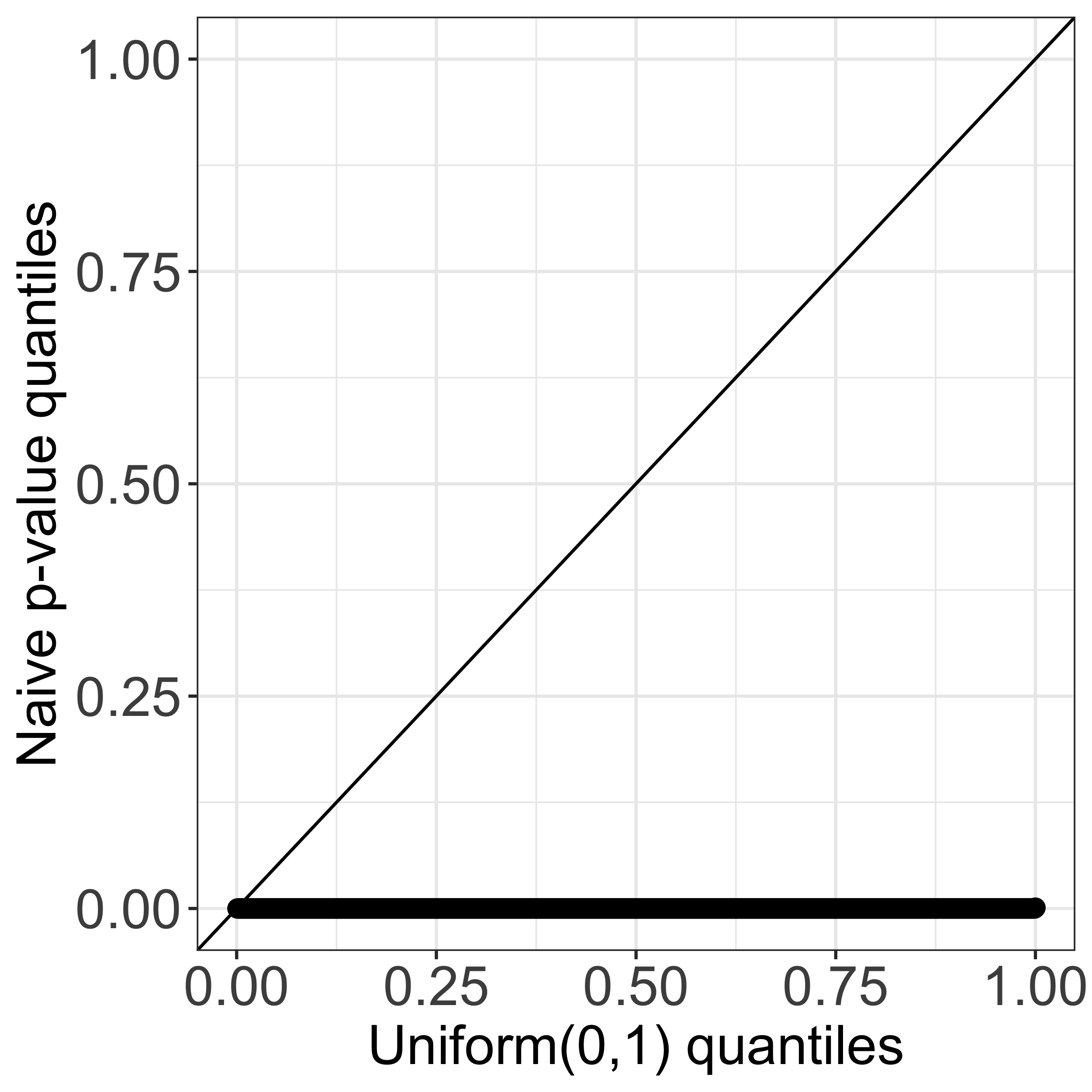
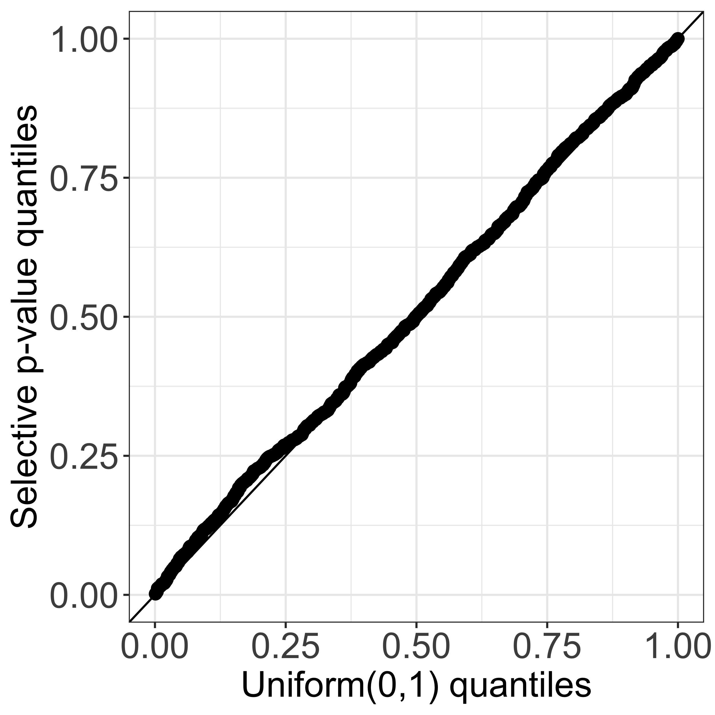
Our software implements an efficient calculation of this \(p\)-value by analytically characterizing the set \(\mathcal{S}_T\). Our key insight is that the set \(\mathcal{S}_T\) can be expressed as the intersection of solutions to \(\mathcal{O}(nKT)\) quadratic inequalities of \(\phi\), where \(n,K,\) and \(T\) are the number of observations, the number of estimated clusters, and the number of iterations of Algorithm 1, respectively. The test based on the resulting \(p\)-value will control the selective Type I error, in the sense of Lee et al. (2016) and Fithian et al. (2014); see also Figure 1(c) of this tutorial. Additional details can be found in Sections 2 and 3 of our paper (Chen and Witten 2022+)).

Remark: by contrast, the Wald \(p\)-value takes the form \[ p_{\text{Naive}} = \mathbb{P}(\Vert \mathbf{X}^{\top}\nu \Vert_2 \geq \Vert \mathbf{x}^{\top}\nu \Vert_2), \] which ignores the fact that the contrast vector \(\nu\) is estimated from the data via \(k\)-means clustering, and therefore leads to a test with an inflated Type I error.

Extensions

Our software also allows for the following extensions:

1. Allow for inference with unknown \(\sigma\), i.e., where \(\mathbf{X} \sim \mathcal{MN}_{n\times q}(\boldsymbol{\mu}, \textbf{I}_n, \sigma^2 \textbf{I}_q)\) with unknown \(\sigma\).
2. Allow for inference with a known, positive-definite covariance matrix \(\boldsymbol{\Sigma}\), i.e., where \(\mathbf{X} \sim \mathcal{MN}_{n\times q}(\boldsymbol{\mu}, \textbf{I}_n, \boldsymbol{\Sigma})\).

References

Chen YT and Witten DM. (2022+) Selective inference for \(k\)-means clustering. arXiv preprint. https://arxiv.org/abs/2203.15267.

Fithian W, Sun D, Taylor J. (2014) Optimal Inference After Model Selection. arXiv:1410.2597 [mathST].

Gao, L. L., Bien, J., and Witten, D. (2020). Selective inference for hierarchical clustering. arXiv:2012.02936.

Lee J, Sun D, Sun Y, Taylor J. Exact post-selection inference, with application to the lasso. Ann Stat. 2016;44(3):907-927. doi:10.1214/15-AOS1371