Software tutorials
Tutorials.RmdIn this tutorial, we demonstrate how to use the GFLassoInference package.
First we load relevant packages:
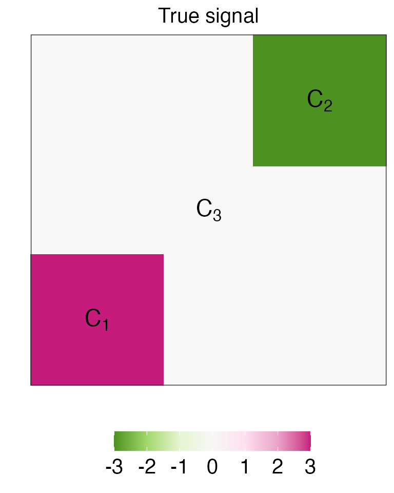
We first construct the signal \(\beta\) that is piecewise constant on an 8 by 8 grid graph, with three true piecewise constant segments taking on values \(-3\), \(0\), and \(3\). We will also use the getD2d function from the genlasso package to create the penalty matrix \(D\) that corresponds to this grid graph.
lev1 <- 0 # mean for group 1
lev2 <- 3 # mean (absolute value) for group 2/3
sigma <- 1 # level of noise
nn <- 8 # grid size
Dmat <- genlasso::getD2d(nn, nn)
# Create the underlying signal
A <- matrix(lev1, ncol=nn, nrow = nn)
A[1:round(nn/3),1:round(nn/3)] <- 1*lev2
A[(nn-2):(nn),(nn-2):(nn)] <- -1*lev2
beta <- c(t(A)) # flatten the matrix by row
The code below visualizes the signal \(\beta\). For convenience, we will refer to the three segments of \(\beta\) as \(C_1\), \(C_2\), and \(C_3\), respectively (colored in magenta, green, and grey in the figure below).
A_true_value_plot <- data.frame(expand.grid(c(1:8),c(1:8)), z = beta)
ggplot(A_true_value_plot, aes(x=Var1, y=Var2, fill = z)) +
  geom_tile() +
  xlab("") + ylab("") +
  ggtitle("True signal")+
  scale_fill_distiller(palette = "PiYG")+
  theme_bw()+
  theme(plot.title=element_text(size=15,hjust = 0.5),
        axis.text.y=element_text(size=15),
        axis.text.x=element_text(size=15),
        legend.position="bottom",
        legend.title = element_blank(),
        legend.text = element_text(size=15),
        axis.title=element_text(size=15),
        strip.text.y = element_text(size=15,hjust=0,vjust = 1,angle=180,face="bold"))+
  scale_x_discrete(expand = c(0,0)) +
  scale_y_discrete(expand = c(0,0)) +
  annotate("text",x = 2 ,y = 2, label = TeX("$C_1$"),parse=TRUE,size=6)+
  annotate("text",x = 7 ,y = 7, label = TeX("$C_2$"),parse=TRUE,size=6)+
  annotate("text",x = 4.5 ,y = 4.5, label = TeX("$C_3$"),parse=TRUE,size=6)+
  guides(fill = guide_colourbar(barwidth = 10, barheight = 1))
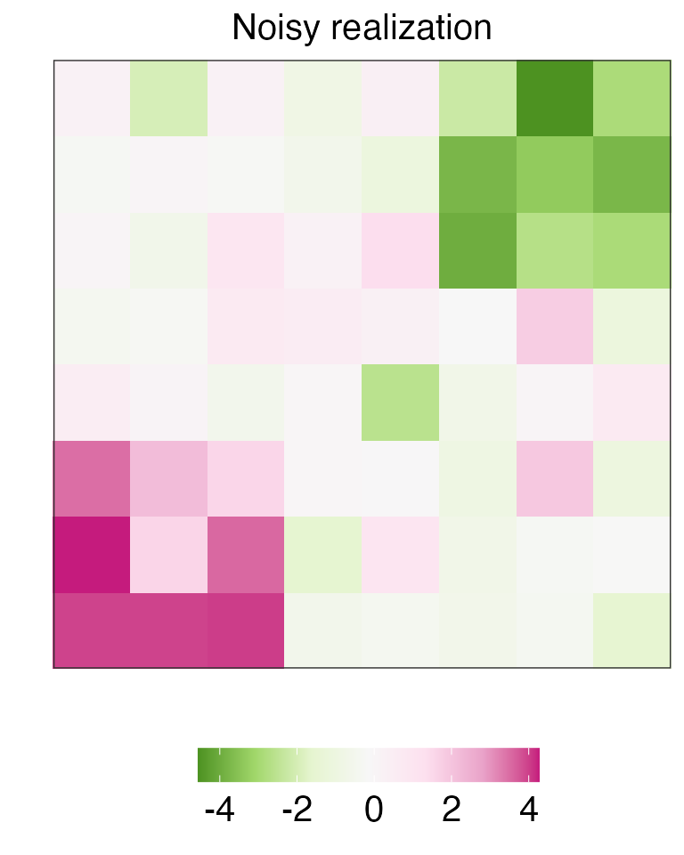
We draw a sample y from the model \(Y_i = \beta_j + \epsilon_j, \epsilon_j \overset{i.i.d.}{\sim} N(0, 1), \; j = 1,\ldots, 64\).
The code below displays the sampled observation y.
A_noisy_value_plot <- data.frame(expand.grid(c(1:8),c(1:8)), z = c(t(A.noisy)))
ggplot(A_noisy_value_plot, aes(Var1, Var2, fill = z)) +
  geom_tile() +
  xlab("") + ylab("") +
  ggtitle("Noisy realization")+
  scale_fill_distiller(palette = "PiYG")+
  theme_bw()+
  theme(plot.title=element_text(size=15,hjust = 0.5),
        axis.text.y=element_text(size=15),
        axis.text.x=element_text(size=15),
        legend.position="bottom",
        legend.title = element_blank(),
        # axis.ticks.y=element_blank(),
        legend.text = element_text(size=15),
        axis.title=element_text(size=15),
        strip.text.y = element_text(size=15,hjust=0,vjust = 1,angle=180,face="bold"))+
  scale_x_discrete(expand = c(0,0)) +
  scale_y_discrete(expand = c(0,0))+
  guides(fill = guide_colourbar(barwidth = 10, barheight = 1))
The graph fused lasso estimator
In the code below, we use the fusedlasso function (see link for detailed documentations of the fusedlasso function) in the genlasso package to obtain the graph fused lasso estimator \(\hat\beta\) on the data y. In this example, we apply the dual path algorithm on y with \(K=13\), which yields three estimated connected components.
K = 13
complete_sol <- genlasso::fusedlasso(y=y,D=Dmat,maxsteps=K)
beta_hat <- complete_sol$beta[,K]
#  estimated connected components
estimated_CC <- complete_sol$pathobjs$i
estimated_CC
#>  [1] 2 2 2 3 3 3 3 3 2 2 2 3 3 3 3 3 2 2 2 3 3 3 3 3 3 3 3 3 3 3 3 3 3 3 3 3 3 3
#> [39] 3 3 3 3 3 3 3 1 1 1 3 3 3 3 3 1 1 1 3 3 3 3 3 1 1 1
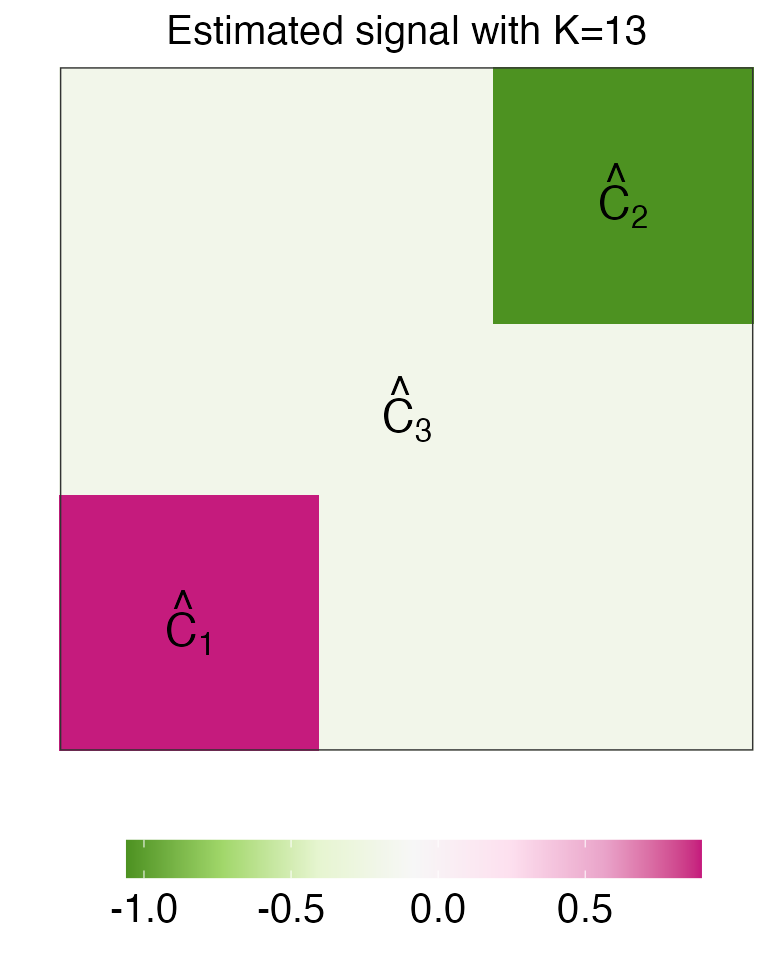
There are exactly three estimated connected components in \(\hat{\beta}\) (referred to as \(\hat{C}_1\),\(\hat{C}_2\), and \(\hat{C}_3\) for convenience). In this case, the fused lasso estimator with \(K=13\) perfectly recover the underlying piecewise constant segments of \(\beta\), where \(\hat{C}_1\), \(\hat{C}_2\), and \(\hat{C}_3\) correspond to the segments of \(\beta\) with mean -3, 0, and 3, respectively.
table(estimated_CC,beta)
#>             beta
#> estimated_CC -3  0  3
#>            1  9  0  0
#>            2  0  0  9
#>            3  0 46  0
The code below displays \(\hat\beta\) and the estimated connected components.
A_estimate_value_plot <- data.frame(expand.grid(c(1:8),c(1:8)), z = c(t(beta_hat)))
ggplot(A_estimate_value_plot, aes(Var1, Var2, fill = z)) +
  geom_tile() +
  xlab("") + ylab("") +
  ggtitle("Estimated signal with K=13")+
  scale_fill_distiller(palette = "PiYG")+
  theme_bw()+
  theme(plot.title=element_text(size=15,hjust = 0.5),
        axis.text.y=element_text(size=15),
        axis.text.x=element_text(size=15),
        legend.position="bottom",
        legend.title = element_blank(),
        legend.text = element_text(size=15),
        axis.title=element_text(size=15),
        strip.text.y = element_text(size=15,hjust=0,vjust = 1,angle=180,face="bold"))+
  scale_x_discrete(expand = c(0,0)) +
  scale_y_discrete(expand = c(0,0))+
    annotate("text",x = 2 ,y = 2, label = TeX("$\\hat{C}_1$"),parse=TRUE,size=6)+
  annotate("text",x = 7 ,y = 7, label = TeX("$\\hat{C}_2$"),parse=TRUE,size=6)+
  annotate("text",x = 4.5 ,y = 4.5, label = TeX("$\\hat{C}_3$"),parse=TRUE,size=6)+
  guides(fill = guide_colourbar(barwidth = 15, barheight = 1))
Graph Fused Lasso Inference
In this section, we demonstrate how to use our software to obtain \(p\)-values and confidence intervals for the difference in means between a pair of estimated connected components. We will use \(\hat{C}_1(y)\) (lower left) and \(\hat{C}_3(y)\) (middle) as an example. Recall that for a given pair of estimated connected components, our proposed \(p\)-value \(p_{\hat{C}_1,\hat{C}_2}\) can be expressed as \(\mathbb{P}\left(|\phi| \geq |\nu^\top y| \;\middle|\; \phi \in \mathcal{S}_{\hat{C}_1,\hat{C}_2}\right),\) where \(\mathcal{S}_{\hat{C}_1,\hat{C}_2}\) is the set of values \(\phi\) such that performing the graph fused lasso on the perturbed dataset \(y'(\phi)\) that yields \(\hat{C}_1(y)\) and \(\hat{C}_3(y)\) (see details in the technical details section).
The code below illustrates the use of fusedlasso_inf, which performs inference on the specified two estimated connected components. The connected components are numbered as per estimated_CC, i.e., the results of the fusedlasso function of the genlasso package. After performing inference with \(K=13\) in this example, we use the summary method to get a summary of the results, in the form of a data frame.
result_demo <- fusedlasso_inf(y=y, D=Dmat, c1=1, c2=3, method="K", sigma=sigma, K=K,
compute_ci = TRUE, alpha_level = 0.05)
summary(result_demo)
#>   CC_1 CC_2 test_stats    pval_c1c2 pval_hyun       LCB       UCB
#> 1    1    3  -3.152508 1.430407e-12 0.2545821 -3.866876 -2.434958
The summary contains the difference in means, i.e., \((\sum_{j \in \hat{C}_1} y_j)/|\hat{C}_1| -(\sum_{j \in \hat{C}_3} y_j)/|\hat{C}_3|\) (test_stats), \(p_{Hyun}\) (pval_hyun), \(p_{\hat{C}_1,\hat{C}_2}\) (pval_c1c2), and an accompanying \((1-\alpha)\) confidence interval based on \(p_{\hat{C}_1,\hat{C}_2}\) ([LCB,UCB]). Because \(p_{Hyun}\) conditions on too much information, the test based on \(p_{Hyun}\) has low power, and therefore cannot reject \(H_0\) at level \(\alpha=0.05\) (\(p_{Hyun}=0.25\)). By contrast, the test based on \(p_{\hat{C}_1,\hat{C}_2}\) can easily reject this null hypothesis (\(p_{\hat{C}_1,\hat{C}_2}<0.001\)).